I. Introduction

Empirical evidence points to 2006 as the “incipient” year in a global trend of “decline in democracy”.^[1] Modern liberal democracies are defined as having three fundamental institutions: the state, which monopolises power to maintain peace, enforce laws, and provide security and basic public goods; the rule of law that constrains the power of the state and the elite; and democratic accountability, whereby free and fair elections ensures that the state works in the interest of the community.^[2] While cross-country comparisons are important to understand current patterns of secular stagnation in democratic systems across the world, it is equally relevant to analyse the state of democracy in specific countries, particularly the low- and middle-income ones.

This paper studies India—the largest democracy in the world with an electorate of more than 900 million. Gender equity in democratic accountability, which is instrumental for civil and political rights,^[3] is an important dimension that needs exploration from the perspective of whether or not the gap has closed or narrowed over time. This paper examines decadal trends (from the first state election in 1951 till 2019) in women’s political empowerment through their participation in the electoral process at three levels: as voters, as contestants, and as winners of elections.

This analysis seeks to complement existing research on gender gaps in political participation in the Indian context, which has primarily limited their attention to women’s election to political positions and their impact on social outcomes. For example, research has shown that women political leaders have a distinct gender effect on the provision of public goods, and on public expenditure;^[4] have led to reduced infant mortality rates;^[5] have improved educational achievements;^[6] and encouraged future political participation of women.^[7] Other research, meanwhile, have either found no impact, or indeed, adverse impacts of women leaders on gender-specific provision of public goods.^[8]

Such exclusive focus on women leaders was also seen in the Global Gender Gap Report of 2017,^[9] which highlighted gender gaps in political empowerment by looking at the ratio of women to men in national parliamentary and ministerial positions.9 Even the Economist democracy index,^[10] while analysing political participation as parameter of democracy, focused on women in parliament. To be sure, however, there is emerging interest in studying women voter turnouts.^{[11],[12],[13],[14]}

To build a more comprehensive understanding of the gender gaps in political empowerment, it is imperative to go beyond women as political leaders, or voters, and expand the analysis to include women as political contestants in elections across the country. This paper conducts a systematic exploration of decadal trends in women’s political empowerment from all three angles: as voters, contestants, and winners in India, from the first state assembly election in 1951 till the most recent election in 2019. The authors collect constituency-level data from state legislative assembly elections, and analyse decadal trends in women’s participation in the electoral process.

First, to study women as voters, the authors trace the curve of the sex ratio (female per 1,000 males) of the electorate (people who are eligible to vote) with the sex ratio of the voters (people who cast their vote). The difference between the two sex ratios reflects gender differences in actual voter participation. Second, to study women as contestants, the authors analyse the likelihood of women contesting elections over time. Third, the authors study women as winners, analysing trends in the likelihood of women winning an election over time.

II. Methodology

1. Outcome variables

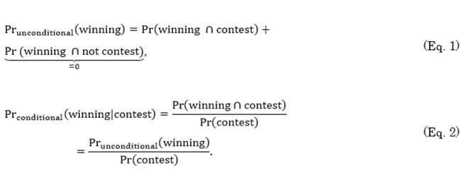
There are three outcome variables that are of interest to this analysis. First, the sex ratio of the electors and the voters. Electors are citizens who are registered to vote, and the sex ratio is the number of female electors per 1,000 male electors. Voters are defined as those who cast their vote in the election, and the sex ratio is the number of female voters per 1,000 male voters. For each constituency, the authors compute the sex ratios of electors and voters. The second outcome at the level of a constituency, is whether there was at least one female contesting in the election. This is a dummy variable that takes value ‘1’ if there was at least one female contestant, and ‘zero’ otherwise. The third outcome of interest is whether the winner of the election was a female or not. For this the authors consider two sub outcomes: (a) unconditional winner, which takes a value of 1 if the women won the election and zero otherwise, irrespective of whether a woman contested the election or not in the constituency; and (b) conditional winner, where the analysis is limited to outcomes only in those constituencies where women contested the election. In particular,

The implications are that over time, more women could be elected because more women are contesting seats. However, the probability of women winning conditional on contesting could decline because over time, the probability of women contesting could rise faster than the probability of women winning the election.

2. Data

This study uses data from the Election Commission of India (ECI). ECI is an autonomous constitutional authority established in 1950, that is responsible for administering elections to the Lok Sabha (national parliamentary elections), Rajya Sabha (upper house of the national parliament), state legislative assembly, state legislative council, offices of the President and the Vice President of India. The analysis is based on the state legislative elections from the period beginning 1951, when the first state elections were held, till 2019. The unit of observation is the constituency, where data is available for gender distribution, (a) of number of candidates contesting, (b) of electors who are registered with the ECI to vote, and (c) of voters who cast their vote.

In its effort to ensure transparency and fairness in the election process, after every election, the ECI makes constituency-level data publicly available on its website in a portable document format. The authors scraped this data from the ECI website. The data on gender distribution of candidates is available for every constituency election. However, data on gender distribution of electors and voters is available only from 1969 onwards. Additionally, there are 166 (0.37 percent) constituency elections for which gender distribution data are not available, of which 132 constituencies were elections with only one contestant so no voting was held. For the remaining 34 constituencies, gender distribution data for electors and voters was not reported by the ECI.

3. Statistical Analysis 

The authors performed statistical analysis at two levels: all-India, and state. For the first outcome, which looks at the sex ratio of voters and electors, the authors run a pooled quantile regression.[a] Using the qreg command from STATA MP 15 (StataCorp 1985-2015), the authors ran the following quantile regression,

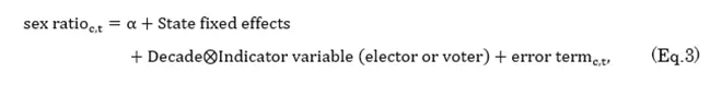
where sex ratio_c,t, is the sex ratio (female per 1000 male) at the level of the constituency c in the year t when the election was held. State fixed effects accounts for unobserved differences that exist across states. , is an interaction term between decade when the election was held and an indicator variable of whether the sex ratio is of electors or voters. The interaction allows for the decadal trends to be different for sex ratio of voters, and of electors.

The gender distribution data for electors and voters is available from 1969 onwards, and therefore, the decades are divided into five: 1970s [1970-79], 1980s [1980-89], 1990s [1990-99], 2000s [2000-09], and 2010s [2010-19]. The error terms are clustered at state and year in which the election was held to account for potential correlations that might exist across constituencies within a state and in that year of election. After running the quantile regressions, the authors use margins command to compute average predicted values for each decade, for electors and voters, respectively. The authors then compute the difference between sex ratio of voters and of electors, and test whether it was statistically different from each other at the conventional 5% level using p values from the chi square test. A similar analysis is performed at the individual state level. ^[15]

For the second, and third outcome, the authors analyse the probability of women contesting election, and of women winning election, respectively, using logistic regression analysis. The authors run the following regression,

where y, is the outcome of interest; (a) whether a woman contested an election, and (b) whether women won the election, respectively, in constituency, c, and in time period, t. State fixed effects, as before, account for unobserved differences that exist across states. The years are divided into seven decades: 1950s [1951-59], 1960s [1960-69], 1970s [1970-79], 1980s [1980-89], 1990s [1990-99], 2000s [2000-09], and 2010s [2010-19]. As before the error terms are clustered at state and year. For logistic regression for women winning an election, the authors run additional logit regression, where data is limited to only those constituencies where women contested the election. The objective of this analysis is to provide empirical trends for conditional probability of women winning an election. After each of the regressions, margins STATA command is used to compute the average predicted probabilities for each of the decades. A similar analysis is conducted for each state.

3. Results

Election results from 55,690 constituencies from 1951 to 2019 were analysed across 31 states and union territories (UTs) in India. Out of 55,690 legislators who were elected, 2,720 (4.9 percent) were women. Of the 55,690 constituencies, 14,522 (26.1 percent) had at least one women contestant. There were 4,55,956 total contestants, of which 20,440 (4.5 percent) were women. The authors find a systematic and significant increase in the proportion of female candidates rising from 1.6 percent in the 1950s to 8.1 percent in the 2010s. Meanwhile, the number of constituencies with at least one female contestant increased substantially from 7.7 percent in the 1950s to 54.1 percent in the 2010s. Similarly, the proportion of women winners rose from 3.9 percent of constituencies in the 1950s to 8.6 percent in the 2010s (see Table 1). (Table S1 shows the results for each election).

Next, the authors examine the decadal trends in the sex ratios of electors and voters. The analysis finds that the sex ratio of electors fell marginally from 939 in the 1970s to 928 in the 2010s. However, the sex ratio of voters increased significantly from 793 to 928. The difference in the sex ratio of voters and electors reduced over time, falling from -146 (P value <0.01) in the 1970s to 0 (P value = 0.76) in the 2010s (see Table 2 & Figure 1). The state analyses are reported in the supplementary tables (Table S2 & Figure S1). The findings show that some of the biggest gains in reduction of gender gap were achieved in less developed states such as Bihar, Odisha, and Uttar Pradesh. In the 2010s the gap between the sex ratio of voters and electors in these states was positive, suggesting a greater female voter turnout compared to men. For Bihar it was 86 (P value <0.01), Odisha was 37 (P value <0.01) and Uttar Pradesh was 25 (P value <0.01). Figure S2 and Figure S3 show trends in male and female voter turnout, across all-India and states, respectively. The authors then compute decadal trends in the odds ratios of at least one woman contesting an election in the constituency. These are based on the logistic regression analysis described earlier in this paper. For odds ratios, the reference period is the 1950s. The findings show that the odds of women contesting elections rose by approximately 16 times in the 2010s as compared to the 1950s. In particular, the odds ratios after adjusting for state fixed effects, was 16.77 (95% CI; 11.65 to 24.14). Similarly, the average predicted probabilities of women contesting an election went up from 7.1% (95% CI; 4.8% to 9.4%) in the 1950s to 54.3% (95% CI; 52.2% to 56.4%) in the 2010s (see Table 3).

The next set of results are decadal trends of women winning elections. The odds ratios are based on unconditional (Eq. 1) and conditional probabilities (Eq. 2). The authors find that compared to the 1950s, the odds of a woman winning an election in a constituency based on unconditional probability of women contesting, were 2.61 times higher in the 2010s, the ORs was 2.61. In terms of average predicted probabilities, women won in 3.6 percent of constituencies in the 1950s, which increased to 8.9 percent in the 2010s. However, in terms of conditional probabilities, the odds of a woman winning an election was 0.18 in the 2010s as compared to the odds in 1950, the ORs was 0.18. In terms of average predicted probabilities, women won in 50.4 percent of constituencies they contested in, while in the 2010s, they won in 15.9 percent. This reduction is primarily driven by an increase in the number of constituencies where women contest elections (see Table 4).

For state analysis of proportion of women contestants and winners, and comparisons with all-India, the results are reported in supplementary figures S2 and S3 (see Figure S4 & Figure S5 for states).

It is important to highlight, however, that the significant surge in women contestants and winners of assembly elections is not uniform across Indian states.  In particular, smaller northeastern states such as Arunachal Pradesh, Manipur, Meghalaya, Mizoram, Nagaland, and Sikkim perform very poorly in terms of women contestants and winners. Ironically, all these states report progressive sex ratios (electors and voters) that are in excess of 1,000 and these states have traditionally reported high proportions of tribal population compared to rest of India. However, each of these states lag behind the all-India numbers in terms of proportions of women contestants and winners of assembly elections. Perhaps an extreme feature of persistent gender inequality in political participation of women is that the state of Nagaland has not elected a single woman legislator till date.

IV. Discussion and Conclusion

Global empirical trends suggest a “mild but protracted democratic recession” since 2006.^[16] This is primarily based on data on political rights and civil liberties from Freedom House. As important as global trends may be, it is equally important to look at whether democratic traditions and institutions are either strengthening or weakening within established democracies, particularly in low- and middle-income countries such as India. With the economic resurgence of authoritarian regimes such as China, there are temptations to sacrifice political rights and civil liberties for economic prosperity. In the context of emerging economies, slow consensus-building processes in their democratic systems could be perceived as hindrance to economic reforms and progress. Yet, from the perspective of promoting individual political rights and civil liberties, democracy is an end in itself, even if it implies in the short run, slow economic growth. Indeed, there is evidence that democracies help nurture long-term economic growth.^[17]

Furthermore, in the context of established large democracies, such as India with its more than 900-million-strong electorate, it is important to go beyond national elections, and focus on state legislative elections. After all, in India’s federal structure, the legislative powers are shared between the center and states. Moreover, the deeper the roots are of democratic traditions at the local level, the more democracy will thrive. ^[18]

This paper, therefore, analysed every state legislative election in India from the beginning, across all states. The aim is to examine the gender gaps that persist in political participation. For example, in the decade of 1950s, out of 3,522 constituencies, there were only 272 (7.7 percent) constituencies with a woman contestant; however, by the 2010s, women contested in some 4,400 out of 8,140 constituencies (54.1%)—representing a nearly seven-fold increase.

In terms of voters, in the 1950s, on average there were 939 females per 1,000 male electors, but in terms of those who actually cast their votes, the ratio was 793 females per 1,000 male voters, or a difference of 146 females per 1,000 males who did not cast their votes. By the 2010s, the gender gap in sex ratio of voters and electors had narrowed to zero, suggesting a steep rise in female voter turnout (Figure S2 and Figure S3). Similarly, in terms of women as election winners, in the 1950s, they won in only 137 (3.9 percent) of the constituencies and by the 2010s, they took seats in 698 (8.6 percent) of the constituencies.

It is important to view these trends from a global perspective: In contrast to global trends that show an apparent decline in democracy since 2006, India is witnessing a strengthening of democratic traditions and institutions in terms of women’s political participation. At the same time, however, one must exercise caution in overestimating the gains—while these robust trends show a clear decline in gender gaps, gender parity is yet to be achieved. Further research is required to understand the underlying causes of these persistent inequities, and how they can be addressed.

This paper argues that there are systematic and comprehensive increasing trends in women’s participation—as voters, contestants, and winners—in the democratic process at the state legislative elections across India. The most impressive gains were made in women’s participation as voters and contestants. These trends are easily missed given the overwhelming focus by the popular media—national and international—on women as winners of elections. The decadal trends in reductions in gender disparity in terms of political rights, in addition to other measures of promoting civil liberties, comprise a more comprehensive and truer reflection of growth in women’s liberty and overall freedom, as well as the strengthening of Indian democracy.

Table 1: Summary

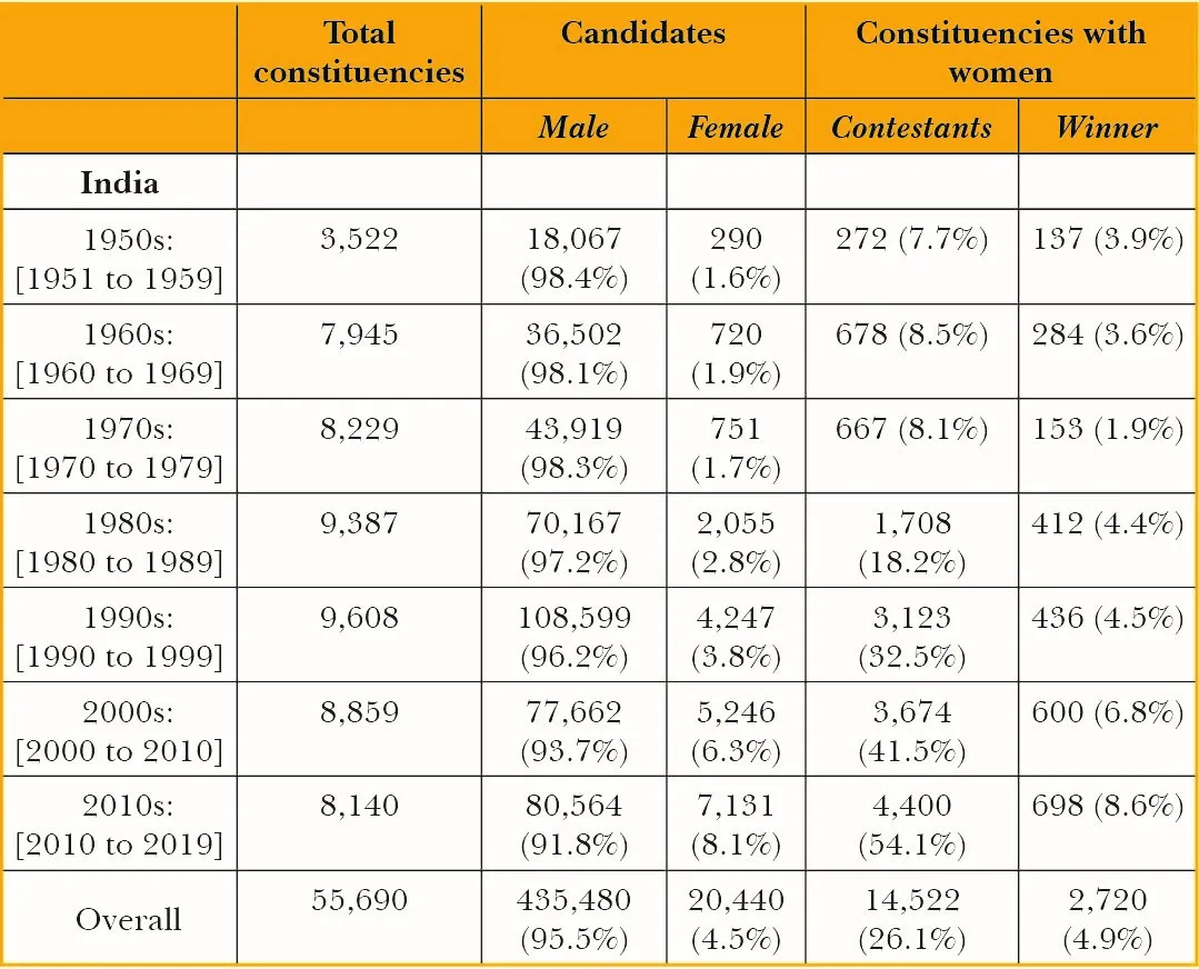
Table 2: Sex ratio (female per 1000 male) of Electors and Voters across decades

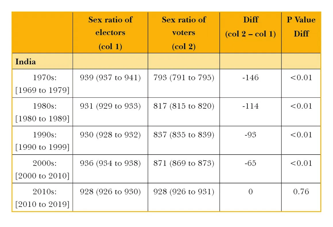
Note: Sex ratio of electors and voters are computed based on a quantile regression, where sex ratio is the dependent variable. Explanatory variables include state fixed effects, to account for unobserved differences in state characteristics, and a dummy variable for each decade interacted with sex ratio was of electors and voters. The p values of differences between sex ratio of electors and voters are computed based on  test of difference.

Figure 1: Difference between sex ratio (female per 1000 male) of voters and electors across decades

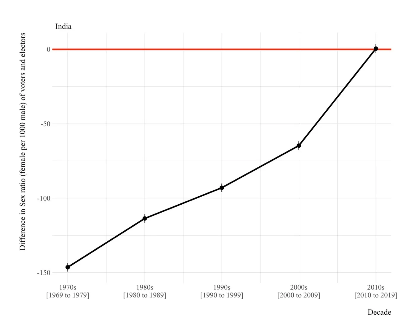
Note: Vertical bars are 95% confidence intervals.

Table 3: Odds Ratios and Average predicted probabilities of women contestants

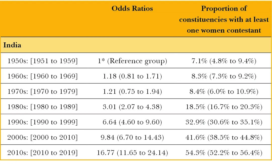
Note: The odds ratios are computed by running a logistic regression at the constituency level where the dependent variable takes a value 1 if there is at least one female contestant contesting an election, and takes a value 0 otherwise. The explanatory variables include state fixed effects, to account for unobserved differences in state characteristics, and a dummy variable for each of the decades, where the decade of 1950s [1951 to 1959] is the reference group. The standard errors are clustered for the state and the year of the election. The proportion of constituencies with at least one contestant are computed as the average predicted probabilities of a female contestant for each of the decades. The 95% confidence intervals are in parenthesis. 

Table 4: Odds Ratios and Average predicted probabilities of women winners

Note: The odds ratios are computed by running a logistic regression at the constituency level where the dependent variable takes a value 1 if women won the election in the constituency, and takes a value 0 otherwise. For the conditional regressions we limit our analysis to those constituencies where women contested the election. The explanatory variables include state fixed effects, to account for unobserved differences in state characteristics, and a dummy variable for each of the decades, where the decade of 1950s [1951 to 1959] is the reference group. The standard errors are clustered for the state and the year of the election. The proportion of constituencies where women won an election are computed as the average predicted probabilities of a female contestant for each of the decades. The 95% confidence intervals are in parenthesis.

Table S2: Sex ratio of Electors and Voters across decades, All India and States 

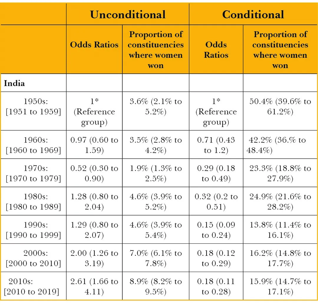
Note: The odds ratios are computed by running a logistic regression at the constituency level where the dependent variable takes a value 1 if women won the election in the constituency, and takes a value 0 otherwise. For the conditional regressions we limit our analysis to those constituencies where women contested the election. The explanatory variables include state fixed effects, to account for unobserved differences in state characteristics, and a dummy variable for each of the decades, where the decade of 1950s [1951 to 1959] is the reference group. The standard errors are clustered for the state and the year of the election. The proportion of constituencies where women won an election are computed as the average predicted probabilities of a female contestant for each of the decades. The 95% confidence intervals are in parenthesis.

Table S2: Sex ratio of Electors and Voters across decades, All India and States 

	Sex ratio of electors (col 1)	Sex ratio of voters (col 2)	Diff (col 2 – col 1)	P Value Diff
India
1970s: [1969 to 1979]	939 (937 to 941)	793 (791 to 795)	-146	<0.01
1980s: [1980 to 1989]	931 (929 to 933)	817 (815 to 820)	-114	<0.01
1990s: [1990 to 1999]	930 (928 to 932)	837 (835 to 839)	-93	<0.01
2000s: [2000 to 2010]	936 (934 to 938)	871 (869 to 873)	-65	<0.01
2010s: [2010 to 2019]	928 (926 to 930)	928 (926 to 931)	0	0.76
Andhra Pradesh
1970s: [1969 to 1979]	1,009 (1,004 to 1,014)	917 (912 to 922)	-92	<0.01
1980s: [1980 to 1989]	1,011 (1,006 to 1,015)	926 (922 to 930)	-85	<0.01
1990s: [1990 to 1999]	1,007 (1,002 to 1,013)	932 (927 to 937)	-75	<0.01
2000s: [2000 to 2010]	1,025 (1,019 to 1,030)	975 (970 to 980)	-49	<0.01
2010s: [2010 to 2019]	1,011 (1,005 to 1,016)	1,002 (996 to 1,007)	-9	0.03
Arunachal Pradesh
1970s: [1969 to 1979]	979 (919 to 1,039)	865 (803 to 927)	-113	0.01
1980s: [1980 to 1989]	948 (905 to 990)	858 (814 to 901)	-90	<0.01
1990s: [1990 to 1999]	925 (900 to 949)	926 (901 to 951)	2	0.93
2000s: [2000 to 2010]	988 (958 to 1,018)	1,035 (1,003 to 1,066)	47	0.04
2010s: [2010 to 2019]	1,021 (991 to 1,051)	1,063 (1,031 to 1,095)	42	0.06
Assam
1970s: [1969 to 1979]	867 (858 to 876)	726 (717 to 735)	-142	<0.01
1980s: [1980 to 1989]	882 (873 to 891)	819 (810 to 828)	-63	<0.01
1990s: [1990 to 1999]	900 (891 to 909)	862 (853 to 871)	-38	<0.01
2000s: [2000 to 2010]	934 (925 to 943)	895 (886 to 904)	-39	<0.01
2010s: [2010 to 2019]	936 (927 to 944)	927 (918 to 935)	-9	0.16
Bihar
1970s: [1969 to 1979]	926 (917 to 935)	566 (557 to 575)	-360	<0.01
1980s: [1980 to 1989]	912 (901 to 923)	619 (608 to 630)	-293	<0.01
1990s: [1990 to 1999]	894 (883 to 905)	707 (696 to 718)	-187	<0.01
2000s: [2000 to 2010]	879 (869 to 889)	731 (721 to 740)	-148	<0.01
2010s: [2010 to 2019]	867 (855 to 880)	949 (937 to 962)	82	<0.01
Chhattisgarh
2000s: [2000 to 2010]	990 (983 to 997)	932 (926 to 939)	-57	<0.01
2010s: [2010 to 2019]	984 (977 to 991)	981 (974 to 987)	-3	0.48
NCT OF Delhi
1970s: [1969 to 1979]	755 (742 to 767)	759 (746 to 772)	4	0.65
1980s: [1980 to 1989]	766 (748 to 784)	782 (764 to 800)	16	0.21
1990s: [1990 to 1999]	798 (787 to 809)	698 (687 to 710)	-100	<0.01
2000s: [2000 to 2010]	791 (780 to 803)	753 (741 to 764)	-38	<0.01
2010s: [2010 to 2019]	811 (800 to 822)	791 (779 to 802)	-20	0.01
Goa
1970s: [1969 to 1979]	1,022 (996 to 1,048)	1,001 (975 to 1,027)	-21	0.27
1980s: [1980 to 1989]	981 (961 to 1,002)	952 (932 to 972)	-29	0.05
1990s: [1990 to 1999]	966 (943 to 989)	934 (911 to 957)	-32	0.05
2000s: [2000 to 2010]	990 (968 to 1,013)	967 (944 to 990)	-23	0.15
2010s: [2010 to 2019]	1,022 (999 to 1,045)	1,086 (1,063 to 1,109)	64	<0.01
Gujarat
1970s: [1969 to 1979]	985 (979 to 992)	825 (818 to 832)	-161	<0.01
1980s: [1980 to 1989]	984 (977 to 990)	795 (789 to 802)	-188	<0.01
1990s: [1990 to 1999]	953 (947 to 958)	831 (825 to 836)	-122	<0.01
2000s: [2000 to 2010]	954 (947 to 961)	858 (852 to 865)	-96	<0.01
2010s: [2010 to 2019]	922 (915 to 929)	863 (856 to 870)	-59	<0.01
Haryana
1970s: [1969 to 1979]	893 (886 to 900)	803 (796 to 810)	-90	<0.01
1980s: [1980 to 1989]	879 (873 to 886)	803 (796 to 809)	-77	<0.01
1990s: [1990 to 1999]	854 (848 to 861)	799 (793 to 806)	-55	<0.01
2000s: [2000 to 2010]	836 (830 to 841)	808 (803 to 813)	-28	<0.01
2010s: [2010 to 2019]	860 (853 to 867)	845 (838 to 851)	-15	<0.01
Himachal Pradesh
1970s: [1969 to 1979]	947 (918 to 976)	826 (797 to 855)	-121	<0.01
1980s: [1980 to 1989]	978 (949 to 1,007)	964 (935 to 994)	-14	0.51
1990s: [1990 to 1999]	976 (952 to 1,000)	960 (936 to 984)	-16	0.36
2000s: [2000 to 2010]	973 (944 to 1,002)	1,019 (990 to 1,048)	46	0.03
2010s: [2010 to 2019]	950 (921 to 979)	1,030 (1,001 to 1,059)	80	<0.01
Jammu & Kashmir
1970s: [1969 to 1979]	861 (838 to 885)	704 (680 to 728)	-157	<0.01
1980s: [1980 to 1989]	859 (836 to 883)	766 (742 to 790)	-93	<0.01
1990s: [1990 to 1999]	863 (832 to 894)	621 (590 to 652)	-242	<0.01
2000s: [2000 to 2010]	904 (882 to 926)	761 (739 to 783)	-143	<0.01
2010s: [2010 to 2019]	901 (870 to 932)	915 (884 to 946)	14	0.54
Jharkhand
2000s: [2000 to 2010]	904 (889 to 919)	801 (787 to 816)	-103	<0.01
2010s: [2010 to 2019]	913 (899 to 928)	957 (942 to 972)	44	<0.01
Karnataka
1970s: [1969 to 1979]	958 (952 to 963)	842 (836 to 848)	-116	<0.01
1980s: [1980 to 1989]	963 (959 to 968)	851 (846 to 855)	-113	<0.01
1990s: [1990 to 1999]	972 (966 to 977)	882 (876 to 888)	-90	<0.01
2000s: [2000 to 2010]	972 (966 to 977)	911 (906 to 917)	-61	<0.01
2010s: [2010 to 2019]	972 (967 to 978)	944 (939 to 950)	-28	<0.01
Kerala
1970s: [1969 to 1979]	1,017 (1,005 to 1,028)	994 (983 to 1,006)	-22	<0.01
1980s: [1980 to 1989]	1,021 (1,012 to 1,030)	1,011 (1,002 to 1,020)	-10	0.11
1990s: [1990 to 1999]	1,039 (1,028 to 1,050)	1,029 (1,018 to 1,041)	-10	0.24
2000s: [2000 to 2010]	1,068 (1,057 to 1,079)	1,022 (1,011 to 1,033)	-46	<0.01
2010s: [2010 to 2019]	1,071 (1,060 to 1,082)	1,086 (1,075 to 1,098)	16	0.05
Madhya Pradesh
1970s: [1969 to 1979]	996 (987 to 1,005)	682 (673 to 691)	-314	<0.01
1980s: [1980 to 1989]	983 (974 to 992)	686 (678 to 695)	-297	<0.01
1990s: [1990 to 1999]	949 (942 to 956)	731 (724 to 739)	-217	<0.01
2000s: [2000 to 2010]	912 (901 to 922)	807 (797 to 817)	-105	<0.01
2010s: [2010 to 2019]	911 (900 to 921)	878 (868 to 889)	-32	<0.01
Maharashtra
1970s: [1969 to 1979]	998 (990 to 1,005)	868 (861 to 875)	-129	<0.01
1980s: [1980 to 1989]	994 (987 to 1,001)	824 (817 to 831)	-170	<0.01
1990s: [1990 to 1999]	950 (945 to 956)	871 (865 to 877)	-79	<0.01
2000s: [2000 to 2010]	928 (921 to 935)	849 (842 to 856)	-80	<0.01
2010s: [2010 to 2019]	908 (901 to 915)	855 (848 to 862)	-54	<0.01
Manipur
1970s: [1969 to 1979]	1,034 (1,018 to 1,051)	1,001 (984 to 1,018)	-34	<0.01
1980s: [1980 to 1989]	1,013 (996 to 1,030)	1,033 (1,016 to 1,050)	20	0.1
1990s: [1990 to 1999]	1,009 (991 to 1,026)	1,029 (1,012 to 1,047)	21	0.1
2000s: [2000 to 2010]	1,060 (1,047 to 1,074)	1,067 (1,053 to 1,080)	6	0.53
2010s: [2010 to 2019]	1,043 (1,026 to 1,060)	1,108 (1,091 to 1,124)	65	<0.01
Meghalaya
1970s: [1969 to 1979]	997 (982 to 1,011)	940 (925 to 955)	-57	<0.01
1980s: [1980 to 1989]	1,005 (990 to 1,019)	946 (931 to 961)	-58	<0.01
1990s: [1990 to 1999]	988 (973 to 1,003)	986 (972 to 1,001)	-2	0.87
2000s: [2000 to 2010]	1,007 (992 to 1,022)	1,016 (1,001 to 1,030)	9	0.4
2010s: [2010 to 2019]	1,010 (995 to 1,024)	1,050 (1,035 to 1,065)	41	<0.01
Mizoram
1970s: [1969 to 1979]	1,021 (1,001 to 1,040)	967 (947 to 986)	-54	<0.01
1980s: [1980 to 1989]	978 (958 to 999)	987 (966 to 1,008)	8	0.58
1990s: [1990 to 1999]	995 (975 to 1,016)	995 (974 to 1,015)	-1	0.96
2000s: [2000 to 2010]	1,013 (993 to 1,034)	1,022 (1,001 to 1,043)	8	0.58
2010s: [2010 to 2019]	1,018 (997 to 1,039)	1,057 (1,037 to 1,078)	40	<0.01
Nagaland
1970s: [1969 to 1979]	917 (899 to 934)	902 (885 to 920)	-15	0.25
1980s: [1980 to 1989]	925 (909 to 942)	905 (888 to 921)	-21	0.08
1990s: [1990 to 1999]	939 (919 to 960)	921 (896 to 947)	-18	0.27
2000s: [2000 to 2010]	954 (934 to 975)	936 (915 to 956)	-19	0.2
2010s: [2010 to 2019]	966 (946 to 986)	997 (976 to 1,017)	31	0.04
Odisha
1970s: [1969 to 1979]	935 (923 to 947)	614 (602 to 626)	-321	<0.01
1980s: [1980 to 1989]	924 (910 to 939)	650 (636 to 665)	-274	<0.01
1990s: [1990 to 1999]	904 (889 to 918)	823 (809 to 838)	-80	<0.01
2000s: [2000 to 2010]	942 (930 to 954)	874 (862 to 886)	-68	<0.01
2010s: [2010 to 2019]	933 (918 to 948)	970 (955 to 985)	37	<0.01
Puducherry
1970s: [1969 to 1979]	977 (965 to 989)	967 (955 to 980)	-9	0.29
1980s: [1980 to 1989]	959 (944 to 974)	961 (946 to 976)	2	0.86
1990s: [1990 to 1999]	949 (937 to 961)	954 (942 to 966)	5	0.56
2000s: [2000 to 2010]	1,035 (1,020 to 1,050)	1,053 (1,038 to 1,067)	18	0.1
2010s: [2010 to 2019]	1,092 (1,077 to 1,107)	1,119 (1,104 to 1,134)	27	0.01
Punjab
1970s: [1969 to 1979]	851 (843 to 860)	812 (804 to 821)	-39	<0.01
1980s: [1980 to 1989]	847 (837 to 858)	826 (816 to 836)	-22	<0.01
1990s: [1990 to 1999]	882 (872 to 892)	818 (808 to 828)	-64	<0.01
2000s: [2000 to 2010]	914 (904 to 924)	898 (888 to 909)	-16	0.03
2010s: [2010 to 2019]	889 (878 to 899)	891 (881 to 901)	3	0.73
Rajasthan
1970s: [1969 to 1979]	945 (935 to 956)	752 (742 to 763)	-193	<0.01
1980s: [1980 to 1989]	934 (924 to 944)	736 (726 to 746)	-198	<0.01
1990s: [1990 to 1999]	903 (894 to 911)	764 (756 to 772)	-138	<0.01
2000s: [2000 to 2010]	910 (900 to 920)	856 (846 to 867)	-53	<0.01
2010s: [2010 to 2019]	901 (891 to 911)	904 (894 to 914)	3	0.66
Sikkim
1970s: [1969 to 1979]	829 (803 to 854)	825 (799 to 850)	-4	0.83
1980s: [1980 to 1989]	918 (900 to 936)	803 (785 to 821)	-115	<0.01
1990s: [1990 to 1999]	949 (931 to 967)	878 (860 to 897)	-71	<0.01
2000s: [2000 to 2010]	938 (919 to 956)	931 (912 to 950)	-7	0.61
2010s: [2010 to 2019]	963 (944 to 981)	958 (940 to 977)	-4	0.74
Tamil Nadu
1970s: [1969 to 1979]	1,005 (998 to 1,012)	912 (905 to 919)	-93	<0.01
1980s: [1980 to 1989]	990 (984 to 996)	930 (924 to 935)	-60	<0.01
1990s: [1990 to 1999]	990 (983 to 996)	921 (914 to 928)	-68	<0.01
2000s: [2000 to 2010]	1,014 (1,007 to 1,021)	945 (938 to 952)	-69	<0.01
2010s: [2010 to 2019]	1,003 (996 to 1,010)	1,004 (997 to 1,011)	1	0.88
Tripura
1970s: [1969 to 1979]	946 (935 to 956)	875 (864 to 885)	-71	<0.01
1980s: [1980 to 1989]	967 (956 to 977)	939 (929 to 949)	-28	<0.01
1990s: [1990 to 1999]	945 (934 to 955)	918 (907 to 928)	-27	<0.01
2000s: [2000 to 2010]	943 (933 to 954)	935 (925 to 945)	-8	0.27
2010s: [2010 to 2019]	961 (951 to 972)	995 (985 to 1,005)	34	<0.01
Uttar Pradesh
1970s: [1969 to 1979]	852 (848 to 856)	667 (662 to 671)	-185	<0.01
1980s: [1980 to 1989]	818 (814 to 822)	666 (662 to 671)	-152	<0.01
1990s: [1990 to 1999]	818 (814 to 822)	667 (663 to 671)	-151	<0.01
2000s: [2000 to 2010]	832 (826 to 837)	709 (703 to 714)	-123	<0.01
2010s: [2010 to 2019]	828 (822 to 833)	852 (847 to 858)	25	<0.01
Uttarakhand
2000s: [2000 to 2010]	977 (939 to 1,015)	944 (906 to 982)	-33	0.22
2010s: [2010 to 2019]	900 (862 to 938)	992 (954 to 1,030)	91	<0.01
West Bengal
1970s: [1969 to 1979]	858 (851 to 866)	734 (726 to 741)	-124	<0.01
1980s: [1980 to 1989]	925 (915 to 936)	870 (859 to 880)	-56	<0.01
1990s: [1990 to 1999]	933 (922 to 943)	895 (885 to 906)	-37	<0.01
2000s: [2000 to 2010]	935 (924 to 945)	893 (883 to 903)	-42	<0.01
2010s: [2010 to 2019]	925 (914 to 935)	932 (921 to 942)	7	0.34
Telangana
2010s: [2010 to 2019]	998 (986 to 1010)	993 (981 to 1005)	-5	0.57

Note: The p values are computed based on  test of difference. 

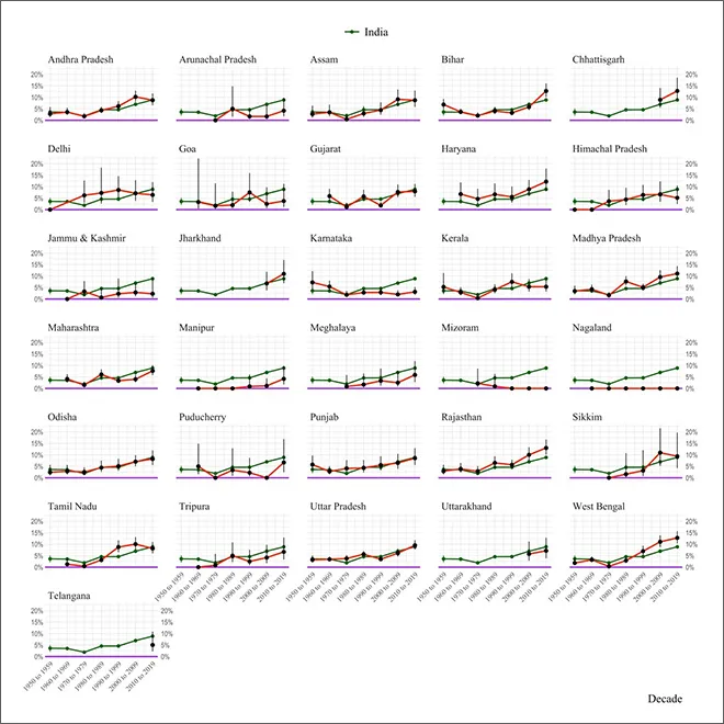
Figure S1: Difference between sex ratio (female per 1000 male) of voters and electors across decades and states in comparison to all-India

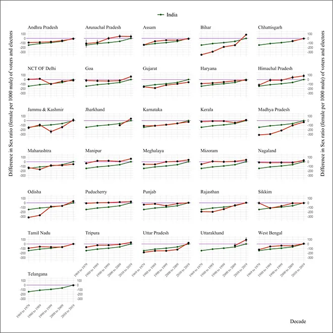
Note: Green line is for all-India. Vertical bars are 95% confidence intervals.

Figure S2: Female and male voter turnout across decades, India

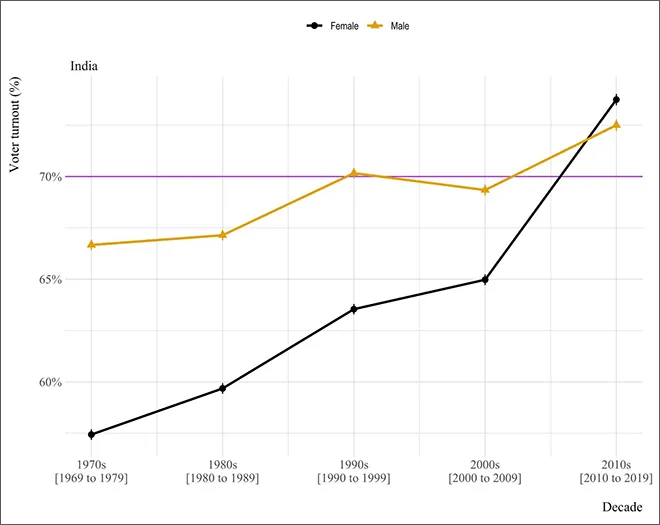
Note: Female and male voter turnout is computed based on a quantile regression, where voter turnout is the dependent variable. Explanatory variables include state fixed effects, to account for unobserved differences in state characteristics, and a dummy variable for each of the decades interacted with whether the voter turnout was for male or female. Purple line is 70% voter turnout; voter turnout >70% reflects strong democratic institutions.10 

Figure S3: Female and male voter turnout across decades and states

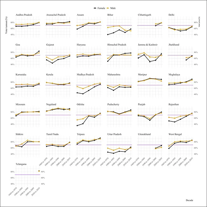
Note: Female and male voter turnout are computed based on a quantile regression, where voter turnout is the dependent variable. Explanatory variables include state fixed effects, to account for unobserved differences in state characteristics, and a dummy variable for each of the decades interacted with whether voter turnout was for male or female. Purple line is 70% voter turnout; voter turnout >70% reflects strong democratic institutions.10 

Figure S4: Proportion of constituencies with at least one female contestant across decades and states in comparison to all-India

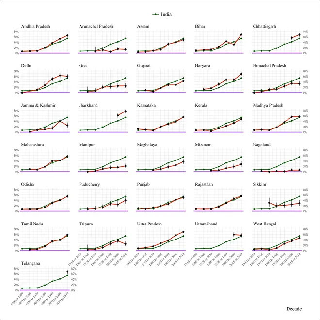
Note: Green line is for all-India. Vertical bars are 95% confidence intervals (CI). The 95% CI are computed using logit transformation so that the end points lie between 0 and 1.

Figure S5: Proportion of constituencies with women as the winner across decades and states in comparison to all-India

Note: Green line is for all-India. Vertical bars are 95% confidence intervals (CI). The 95% CI are computed using logit transformation so that the end points lie between 0 and 1.

Endnotes

• Domestic Politics and Governance
• National Politics
• India
• gender
• India
• occasional papers
• Political Economy
• Skilling

The views expressed above belong to the author(s). ORF research and analyses now available on Telegram! Click here to access our curated content — blogs, longforms and interviews.