
-
CENTRES
Progammes & Centres
Location
 PDF Download
Nilanjan Ghosh and Renita D’ Souza, “Investigating the Impact of Commodity Transaction Tax on India’s Commodity Derivatives Markets,” ORF Occasional Paper No. 313, May 2021, Observer Research Foundation.
1. Introduction
The Commodity Transaction Tax (CTT) became applicable in the Indian commodity derivatives markets beginning 1 July 2013. In the Union Budget speech of 2013, then Finance Minister P Chidambaram noted, “There is no distinction between derivative trading in the securities market and derivative trading in the commodities market, only the underlying asset is different. It is time to introduce Commodities Transaction Tax (CTT) in a limited way. Hence, I propose to levy CTT on non-agricultural commodities futures contracts at the same rate as on equity futures that is at 0.01% of the price of the trade.”[1] Earlier studies have claimed that securities derivatives and commodity derivatives have divergent purposes, with the latter having a wider economy-wide impact.[2] The finance ministry, however, did not share the same view.
Such a tax is imposed to reduce the speculative volumes in the commodity derivatives markets and garner revenues,[3] although the government has not made an explicit declaration of such rationale.[4] The question is whether the tax has indeed helped curb volatility and speculation in the futures markets, or increase government tax revenues.[5] Market participants argue that India’s commodity market has one of the highest ‘cost-per-trade’ rates in the world, and asked Finance Minister Nirmala Sitharaman to reconsider the levy of the CTT in the 2020-21 Union Budget.[6] Earlier, in January 2021, the Commodity Participants Association of India (CPAI) urged the government to rationalise commodities transaction taxes in order to boost trading volumes. In a presentation made to the finance ministry that month, CPAI proposed to treat the CTT as tax paid under section 88E and not as an expense.[7] Yet, the 2021-22 Union Budget—which delved into other development issues—remained silent on the CTT.[a]
In 2002, national-level commodity derivatives exchanges were started in India with the aim of price risk management or hedging, and price discovery.[8] While the former is supposedly a micro-level function of the commodity markets, price discovery is macro-level.[9] Assuming that these remain the fundamental objectives, the efficacy of the commodity derivatives markets in India needs to be assessed through their prisms.
The process of price discovery translates the available information into an asset’s fundamental price.[10] The efficacy of price discovery depends on how swiftly trading responds to the arrival of new information. The ability of the market to discover prices underwrites hedging effectiveness.[11] Axiomatically, the CTT increases the transaction cost of operating in the futures market. It therefore disrupts the in-built stabilisation mechanism of the futures market by crowding out the market players, in turn eroding its efficiency in terms of both price hedging and price discovery.[12] Such arguments were ubiquitous long before CTT was imposed.
To be sure, the logic of having a transaction tax on stock exchanges cannot apply on commodity exchanges, as these two markets have different economic objectives. Participants in the stock markets aim to maximise their profits from the expected rising stock values and participate in derivatives segments with a similar objective. Those who trade in commodity futures, meanwhile, would like to hedge their price risks in fluctuating markets, depending on their physical or cash market exposures. While farmers, merchants, stockists, and importers hedge their stocks and forward purchases against a possible price fall, processors, manufacturers, exporters and even traders with forward sale commitments require hedging against probable adverse price increase.[13] Hedging is an act of protecting a business or an individual from unforeseen losses under conditions of uncertainty of markets that are increasingly exposed to vagaries of international trade and finance. Therefore, a transaction tax on such hedging is tantamount to taxing an insurance mechanism.[14]
On the other hand, price discovery by a futures market also has a much more fundamental role in the context of commodities than in the case of stocks. For futures markets to be efficient, it should not only have a close relation with the physical markets and thereby help hedging through a process of arbitrage between both the markets, but it should also serve as a forum whose prices should be taken as a “reference price” by physical market functionaries.[b] Both these services are contingent upon a sufficient amount of liquidity in the derivatives markets. Therefore, it is unlikely that a thin market will be in a position to discover prices, or even efficiently help in hedging[15] – rather it creates possibilities of speculative trading.[16]
Therefore, any transaction tax imposed on the markets that increase the cost of proprietary trading by more than 300 percent, and client trading by more than 30 percent, will not only disincentivise participation, but also render markets inefficient, at least axiomatically.[17] While CTT’s main purpose may be to discourage speculation, the in-built stabilisation mechanism of the futures market gets distorted and its efficiency gets adversely affected. The CTT adds to the transaction cost of operating in the futures market, eventually crowding out the market players.[18] What is often not understood is the role of speculators in hedging.
Apart from curbing volatility and speculative activity, the CTT, according to government, will bring parity between the commodity and securities markets which are different in their objectives and functioning .[19] Futures markets transactions amount to a zero-sum game for both hedgers and speculators since increments accrued in one period are neutralised by losses in another, while profits for some are cancelled out by losses for others.[20]
Therefore, despite market participants’ long-standing plea to lift the CTT on non-agricultural commodity derivatives, the appeal has gone unheeded. In the Union Budget 2020-21, the CTT was extended on the sale of index futures and options in goods.
This paper investigates the impacts of the CTT on the commodities futures market eight years since its imposition. It studies the cases of aluminium, copper, gold, silver, and crude oil. The paper hypothesises that the traded volume and liquidity have declined and the volatility has increased, and that there will likely be a negative impact on the functions of price discovery and hedging efficiency of the futures market. It examines the revenue impact of the CTT on the exchequer.
Section 2 reviews existing studies that have attempted to assess the impact of transactions tax on market quality, price discovery, and hedging effectiveness. Section 3 describes the data and the methodology employed for the analysis, and Section 4 discusses the results. The paper closes with an outline of the policy implications.
2. Impacts of transaction taxes on markets: Exploratory studies
The impacts of a transaction tax on global financial markets have been studied in various settings. Keynesian and neo-Keynesian approaches have endorsed the imposition of a tax on financial transactions to curb speculative trading. Beginning from Keynes (1936), to Tobin (1978) and Stiglitz (1989), this school advocated that a tax on financial transactions would disincentivise speculation and ensure stability of the financial markets.[21] Summers and Summers (1989) asserted that the benefits of financial stability brought about by the tax would outweigh the decline in liquidity and rise in transaction costs.[22]
Other studies have argued the contrary. In a study on the impact of transaction taxes on volatility, Ross (1989) found an inverse though insignificant correlation between transaction tax and volatility for a sample of 23 countries spanning the period from January 1987 to March 1989.[23] Similarly, while studying financial transaction taxes in Swedish markets, Umlauf (1993) concluded that while there was no dip, rather an increase in the volatility, stock returns and traded volume declined due to the tax.[24] According to Kupiec (1995), the transaction tax distorts information efficiency of markets by discouraging information traders from trading.[25] Saporta and Kan (1997) also found a decline in returns following an increase in transactions costs. Hu (1998) supported this finding.[26] Chou and Lee (2002) demonstrated how transaction taxes adversely affect price discovery, decrease liquidity while increasing volatility.[27]
Lo, Mamaysky, and Wang (2004) corroborated the decline in traded volume due to a rise in transactions costs.[28] Hayashida and Ono (2011) echoed this result.[29] Baltagi, Li, and Li (2006) found both a dip in traded volume and market efficiency following an increase in transactions costs.[30] Chou and Wang (2006) supported a rise in traded volume along with a fall in the bid-ask spread as a result of a reduction in the transaction tax.[31] The study undertaken by Pomeranets and Weaver (2011) corroborated the findings of Chou and Wang.[32] Su and Zheng (2011) demonstrated a negative relationship between the imposition of a transaction tax and traded volume. They found an increase in volatility irrespective of a rise or decline in the transaction tax. While an increase in transaction tax has mixed effects on market efficiency, a decline either brings about a reduction or has no effect in the same.[33]
In the Indian context, Sahoo and Kumar (2008) devised a structural equation model to investigate the effect of a rise in transaction cost on the traded volume and price volatility. The Bid-Ask Spread was made to stand as a proxy for transaction cost. Their investigation concluded a positive relationship between the transactions cost and volatility, as well as between traded volume and volatility, and a negative relationship between the transactions cost and traded volume.[34] The study by Sehgal and Ahmad (2013) found a negative relationship between transaction costs and traded volume, and found a positive correlation between Bid-Ask Spread and intra-day volatility.[35] Ray and Malik (2014) undertook a 50-day and 120-day event study to gauge the impact of CTT on the total volume traded as well as on the market efficiency of the commodity market. The event study concluded a significant dip in traded volume.[36] Sinha and Mathur (2015) also found a decrease in traded volume following an increase in transaction taxes.[37]
Mukherjee (2017) examined the influence of the Commodity Transaction Tax on the health of the commodity futures market from the point of view of turnover, trading costs, Bid-Ask Spread, and other such parameters of market quality. The examination revealed an adverse impact on all aspects of market health. The study concluded that the negative impact of the tax was so severe that the market would not be able to resume its original position.[38] Shanmugam and Champramary (2016) utilised the bootstrap, and modified GARCH methodology to assess the impact of CTT to find an increase in the price volatility in gold futures and reduced traded volume, weakening the market and reducing its efficiency.[39] Sehgal and Agrawal (2019) assessed the impact of CTT on market liquidity and volatility to find a decline in market liquidity, increase in volatility and significant trade migration.[40]
3. Methodology<a style="color: #0069a6;" href="#_ftn3" name="_ftnref3"><sup>[c]</sup></a> and Data Gathering
This study fills a gap in existing literature and examines the impact of CTT on certain variables reflecting on market efficiency—primarily, hedging efficiency and price discovery. It finds important implications for policymakers. The analysis uses open-access daily trading data from January 2006 to December 2019 of Multi Commodity Exchange of India for five non-agricultural commodities: aluminium, copper, crude oil, gold, and silver.[d] Data was taken from the website of the Exchange.
The daily spot prices data from January 2006 to December 2019 was also obtained from the website. The paper defines the pre-CTT period as the seven years and six months prior (1 January 2006 to 30 June 2013), while post-CTT is the six-year six-month period from 1 July 2013 to 31 December 2019.
First, to formulate an appropriate statistical specification for the stochastic processes underlying these variables: are these variables Independent and Identically distributed? Assessing the Identical distribution assumption for all the commodities, regression-based tests are used to unearth deviations from the characteristic of mean homogeneity.[41] Applying the regression:
Xt=α0+ α1t +et
The results are given in Tables 1 and 2 in Appendix 1.
Next, the dependence characteristic of the stochastic processes underlying the variables of volume traded and turnover is assessed by examining the graph of their Auto-Correlation Function. The Box-Pierce tests are also used to generate further evidence for the assessment in question.[42]
To then investigate the effect of CTT on daily volume traded and the daily turnover of the five chosen commodities: The regression models employed in these tests will be based on the statistical information that surfaced from the assessment of the identical distribution and dependence assumptions of the variables volume and turnover.
Running the following regression to gauge the impact of CTT on volume traded:
Vt =β0+ β1 Vt-1 + β2 Vt-2 + β3 Vt-3 + β4 Vt-4+ β5 Vt-5 + β6 Vt-6 + β7 t + β8 Dt (1)
Where:
Dt: Dummy variable which takes the value zero in the pre-CTT period and the value one
in the post-CTT period
Vt: Daily volume traded on day t
Vt-k: Daily volume traded on day t-k(lag of order k)
t: Trend term to capture mean heterogeneity
The following regression is run to gauge the impact of CTT on turnover:[e]
TOt=β0+ β1TOt-1 + β2TOt-2 + β3TOt-3 + β4TOt-4+ β5TOt-5 + β6TOt-6 + β7 t + β8 Dt (2)
Where:
Dt: Dummy variable which takes the value zero in the pre-CTT period and the value one
in the post-CTT period
TOt: Daily turnover on day t
TOt-k: Daily turnover on day t-k(lag of order k)
t: Trend term to capture mean heterogeneity
Liquidity in this exercise has been computed through the Hui-Heubel liquidity ratio defined as follows:[43]
Hui-Heubel Liquidity Ratio = (Highest Price – Lowest Price)/Lowest Price
Turnover/ (Open Interest x Average Price)
The higher the ratio, the lower the liquidity in the market. This implies that even significant price fluctuations are accompanied by minor fluctuations in traded volume.
Just as in the case of the traded volume and turnover, an appropriate statistical specification for the stochastic process underlying the Hui-Heubel Ratio is formulated. First, by examining the characteristic of mean homogeneity by employing the regression-based test of the same form used in the case of traded volume and turnover. This assessment is made for the case of all of the five chosen commodities. The results of this regression for various commodities are shown in Table 7 in Appendix 1.
To examine the dependence characteristic underlying the Hui-Heubel Liquidity Ratio, the Auto-Correlation Functions is evaluated as well as the Box-Pierce tests for the various commodities. The results of this exercise are in Appendix 1 (Figures 11-15 and Table 8).
The regression model used for examining the impact on liquidity for each commodity will depend upon the statistical information about the Hui-Heubel liquidity ratio associated with these commodities.
For example, aluminium exhibits both mean heterogeneity and auto-regressive behaviour though the latter is rather mild compared to the volume and turnover variables. Depending on the auto-regressive behaviour, lag one is added, and lag two and lag six. The following regression is then run:
HHt=β0+ β1HHt-1 + β2HHt-2 + β3HHt-6 + β4t + β5 Dt (3)
In consonance with the autoregressive behaviour of copper in the context of liquidity, the following regression is run to examine the impact of CTT on liquidity:
HHt=β0+ β1HHt-6+ β2t+ β3 Dt (4)
HHt=β0+ β1t+ β2 Dt (5)
HHt=β0+ β1HHt-6+ β2 Dt (6)
HHt=β0+ β1HHt-1 + β2HHt-2 + β3HHt-3 + β4HHt-4+ β5HHt-5 + β6HHt-6 + β7 Dt (7)
Where, in regression equations (3)- (7):
Dt: Dummy variable which takes the value zero in the pre-CTT period and the value one
in the post-CTT period
HHt:Hui-Heubel liquidity ratio on day t
HHt-k: Hui-Heubel liquidity ratio on day t-k(lag of order k)
t: Trend term to capture mean heterogeneity
In order to assess the impact of CTT on the volatility in the futures market of the five commodities, volatility is computed, using the following formula:[44]

Since there is a need to define a statistical specification for the process of volatility for all commodities, the same tests as above will be conducted. The results of these tests are in Appendix 1 (Figures 16-20, and Tables 14 and 15). Based on these results, the following common regression equation is used to check the impact of CTT on the volatility in the futures markets of the chosen commodities.
VVt=β0+ β1VVt-1 + β2VVt-2 + β3VVt-3 + β4 VVt-4+ β5VVt-5 + β6VVt-6 + β7 t + β8 Dt (8)
Where:
Dt: Dummy variable which takes the value zero in the pre-CTT period and the value one in the post-CTT period
Vt: Daily volatility on day t
Vt-k: Daily volatility on day t-k(lag of order k)
t: Trend term to capture mean heterogeneity
Perfectly efficient markets that quickly synthesise new information into price rule out profitable arbitrage. Therefore, new information should be immediately reflected in spot and futures prices by inducing trading in one or both markets simultaneously.[45] Transaction costs tend to be lower in the futures markets as compared to the spot markets. Transaction costs influence the ability to profitably trade on new information. Thus, the adjustment of prices to information is likely to be faster in the futures markets than the spot markets.[46]
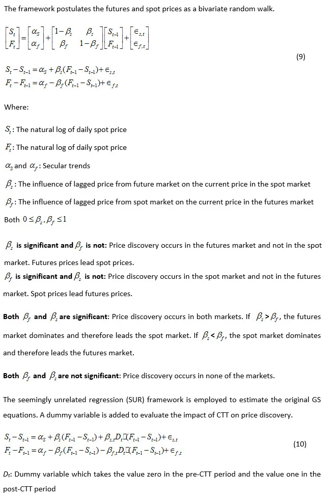
This paper investigates the CTT’s impact on this important function of price discovery in the futures market. After all, the imposition of CTT implies an increase in transactions cost. The question this analysis seeks to answer is whether the ability of the futures markets to respond to new information to incorporate the same into prices by triggering trade has been affected by the levy of the CTT. The authors use the Garbade Silber framework to evaluate whether there exists a functional relationship between the transition in the basis of the previous period and the transitions in the spot or futures prices of the current time period. If the transition in the basis is indeed correlated with the transition in the futures prices, then price discovery occurs in the spot market. If the transition in the basis is indeed correlated with the transition in the spot markets, then price discovery takes place in the futures market.[47]
Hedging against price fluctuations using derivatives has become one of the popular mechanisms of managing risks today. Hedging involves taking equal and opposite positions in the spot and futures markets simultaneously to offset risk. Thus, institutions like the MCX have assumed importance in the context of risk management.[49] This paper’s concern is whether the imposition of the CTT has affected the efficiency of the hedging function of MCX as regards the five commodities chosen. For this purpose, the query is assessed in a quantitative manner using the following methodology. The changes in spot prices are regressed on the changes in futures prices. the R-squared of the regression measures the hedging efficiency: the greater the R-squared, the greater the hedging efficiency.[h] Hedging efficiency measures the extent to which gains/losses in the spot market are offset by the same in the futures market.[50]
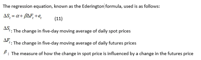
To assess the impact of the CTT on the hedging ratio, the Chow test is conducted to check whether a structural change had occurred in the post-CTT period as compared to the pre-CTT period in the hedging scenario. Within the framework of the Chow test, the above regression is first conducted for the pre-CTT years and then for post-CTT, and the R-squared values for the two regressions are then compared. This comparison will tell whether the hedging efficiency in the futures markets has changed and in which direction, or a status quo remains post- CTT.
4. Results and Analysis
4.1 Impact on volume and turnover traded in the commodities futures market
First, to tabulate the change in average daily turnover due to the imposition of CTT.
Table 4: Change in average daily turnover from pre-CTT years
| Commodity | Aluminium | Copper | Crude oil | Gold | Silver | Combined |
| Average daily turnover in 2011 (₹ crore) | 256.32 | 4116.86 | 6978.04 | 9435.35 | 12321.79 | 33108.35 |
| Average daily turnover in 2017 (₹ crore) | 372.35 | 1323.19 | 3990.27 | 2425.39 | 1725.91 | 9837.11 |
| % change in daily turnover in current prices | 45.27 | -67.86 | -42.82 | -74.29 | -85.99 | -70.29 |
Table 4 shows that volumes in 2017 declined substantially as compared to 2011, a representative year prior to the imposition of CTT, and a normal year prior to the MCX going for its IPO. For the non-agricultural segment, the overall decline is around 70 percent. Given that the non-agricultural segment constitutes more than 80 percent of turnover, there is a high likelihood of revenue loss than increase in revenue from the imposition of the CTT for the government.
The results shown in Tables 1 and 2 lead to the conclusion that all the stochastic process underlying the volume traded and turnover (except copper) for all commodities exhibit mean heterogeneity. Therefore, a trend variable must be included in the regression analysis examining the impact of CTT on volume traded and turnover.
A check for the Auto-correlation functions is done (see Figures 1 to 10 in Appendix 1) over volume and turnover. The ACF of all the commodities viz. aluminium, copper, crude oil, gold and silver, for both their volume traded and turnover, clearly exhibits strong auto-regressive behaviour. The results of the Box-Pierce test in Table 3 of Appendix 1 lend credence to the ACFs of the various commodities. To capture this behaviour, lags up to order six are included in the regression analysis examining the impact of CTT on volume traded and turnover.
The results of the regression analysis in Tables 5 and 6 show that the volumes traded and the turnover, respectively, have declined on account of the imposition of the CTT in the case of all commodities.
Table 5: Regression results: Impacts of CTT on volumes
| Estimate | Aluminium | Copper | Crude Oil | Gold | Silver |
| β0 | -166.4 (469.6) | 5537*** (1147) | 4.830*** (192) | 6386*** (840.3) | 156.40076*** (25.98519) |
| β1 | 0.2812*** (0.01446) | 0.102*** (0.01214) | 0.1675*** (0.01422) | 0.1066*** (0.01300) | 0.12729*** (0.01292) |
| β2 | 0.1176*** (0.01514) | 0.0405*** (0.01222) | 0.05737*** (0.01447) | 0.05384*** (0.01304) | 0.03958** (0.01302) |
| β3 | 0.04391** (0.01524) | 0.01023 (0.01223) | 0.00471 (0.01450) | 0.01532 (0.01306) | 0.01991 (0.01303) |
| β4 | 0.03307* (0.01524) | -0.002476 (0.01223) | 0.004364 (0.01450) | -0.02126 (0.01306) | -0.01213 (0.01302) |
| β5 | 0.01517 (0.01514) | 0.05431*** (0.0122) | 0.05013*** (0.01446) | 0.07928*** (0.01303) | 0.07006*** (0.01301) |
| β6 | 0.4157*** (0.01447) | 0.6441*** (0.01211) | 0.5490*** (0.01419) | 0.5727*** (0.01297) | 0.58018*** (0.01288) |
| β7 | 1.607*** (0.4102) | 4.513*** (0.8807) | 1.429*** (0.2201) | 0.2191 (0.3384) | 0.06703*** (0.01539) |
| β8 | -1862* (822) | -14340*** (2333) | -1942*** (375.8) | -4709*** (906.2) | -286.67786*** (44.39634) |
Level of Significance codes: 0 ‘***’ 0.001 ‘**’ 0.01 ‘*’ 0.05 ‘.’ 0.1 ‘ ’ 1 Standard error in parentheses
Table 6: Regression results: Impacts of CTT on turnover
| Estimate | Aluminium | Copper | Crude Oil | Gold | Silver |
| β0 | -462 (589.8) | 12520*** (3691) | -8644 (7704) | 38650*** (10970) | 10870 (8813) |
| β1 | 0.3524*** (0.01507) | 0.09023*** (0.01187) | 0.1901*** (0.01351) | 0.1335*** (0.01302) | 0.1496*** (0.01256) |
| β2 | 0.1554*** (0.01608) | 0.03451** (0.01921) | 0.03457* (0.01364) | 0.07648*** (0.01311) | 0.06510*** (0.01274) |
| β3 | 0.03801* (0.01625) | 0.009974 (0.01193) | -0.01076 (0.01364) | 0.03510** (0.01316) | 0.03936** (0.01278) |
| β4 | 0.04573** (0.01625) | 0.001415 (0.01913) | -0.002793 (0.01363) | -0.02886* (0.01315) | -0.01473 (0.01278) |
| β5 | -0.007058 (0.01608) | 0.05257*** (0.01190) | 0.03946** (0.01361) | 0.07895*** (0.01310) | 0.06462*** (0.01274) |
| β6 | 0.3178*** (0.01508) | 0.6636*** (0.01183) | 0.6062*** (0.01343) | 0.5724*** (0.01297) | 0.6109 *** (0.01255) |
| β7 | 2.006*** (0.4993) | 21.30*** (3.584) | 86.37*** (10.38) | 38.85*** (8.212) | 29.29*** (7.778) |
| β8 | -0.001883. (1008) | -58460*** (9004) | -139800*** (18280) | -112800*** (20440) | -87170*** (19900) |
Level of Significance codes: 0 ‘***’ 0.001 ‘**’ 0.01 ‘*’ 0.05 ‘.’ 0.1 ‘ ’ 1 Standard error in parentheses
The stochastic process underlying the Hui-Heubel Ratio differs for each of the commodities chosen for analysis. This difference is captured in the variation of the regression models used for examining the impact on liquidity in each of these commodity markets.
As Tables 9, 10, 11 and 13 suggest, the regression co-efficient of the tax dummy variable is positive and statistically significant for aluminium, copper, crude oil and silver. This indicates that the Hui-Heubel liquidity ratio in the post-CTT period has increased in comparison to the pre-CTT period. This means that the liquidity has decreased in the post-CTT period as compared to the pre-CTT period in the case of aluminium, copper, crude oil and silver.
In gold, the sign of the regression co-efficient associated with the tax dummy variable is positive, implying a decline in liquidity. However, the magnitude of the coefficient is statistically significant at 10 percent level of significance, indicating weak evidence of decline in liquidity. The null hypothesis cannot be rejected: that there is a deviation from the pre-CTT levels of liquidity at significance levels below 10 percent.
Overall, the impact of CTT on the liquidity of the futures markets of most commodities expect gold (which also demonstrated a dip in liquidity at 10 percent level of significance) was negative in that the markets experienced a fall in liquidity.
Table 9: Regression results: Impact of CTT on liquidity for aluminium
| Estimate | β0 | β1 | β2 | β3 | β4 | β5 |
| For HH | 3.9292078*** (0.2869920) | 0.0340988* (0.0152022) | 0.0332125* (0.0152019) | 0.3242277*** (0.0151991) | -0.0013752*** (0.0001856) | 0.82183618* (0.4014100) |
Level of Significance codes: 0 ‘***’ 0.001 ‘**’ 0.01 ‘*’ 0.05 ‘.’ 0.1 ‘ ’ 1 Standard error in parentheses
Table 10: Regression results: Impact of CTT on liquidity for copper
| Estimate | β0 | β1 | β2 | β3 |
| For HH | 0.8345*** (0.05305) | 0.5431*** (0.01321) | -.0002160*** (0.00003445) | 0.1646* (0.07874) |
Level of Significance codes: 0 ‘***’ 0.001 ‘**’ 0.01 ‘*’ 0.05 ‘.’ 0.1 ‘ ’ 1 Standard error in parentheses
Table 11: Regression results: Impact of CTT on liquidity for crude oil
| Estimate | β0 | β1 | β2 |
| For HH | 16.320867*** (4.939603) | -0.008759* (7.760585) | 16.075854* (0.003661) |
Level of Significance codes: 0 ‘***’ 0.001 ‘**’ 0.01 ‘*’ 0.05 ‘.’ 0.1 ‘ ’ 1 Standard error in parentheses
Table 12: Regression results: Impact of CTT on liquidity for gold
| Estimate | β0 | β1 | β2 |
| For HH | 3.77046*** (0.16024) | 0.43321*** (0.01432) | 0.33829. (0.01432) |
Level of Significance codes: 0 ‘***’ 0.001 ‘**’ 0.01 ‘*’ 0.05 ‘.’ 0.1 ‘ ’ 1 Standard error in parentheses
Table 13: Regression results: Impact of CTT on liquidity for silver
| Estimate | β0 | β1 | β2 | β3 | β4 | β5 | β6 | β7 |
| For HH | 0.58915*** (0.10503) | 0.08239*** (0.01586) | 0.09566*** (0.01587) | 0.08402*** (0.01594) | 0.02802 . (0.01594) | 0.06763*** (0.01587) | 0.08137*** (0.01585) | 0.58702*** (0.15690) |
Level of Significance codes: 0 ‘***’ 0.001 ‘**’ 0.01 ‘*’ 0.05 ‘.’ 0.1 ‘ ’ 1 Standard error in parentheses
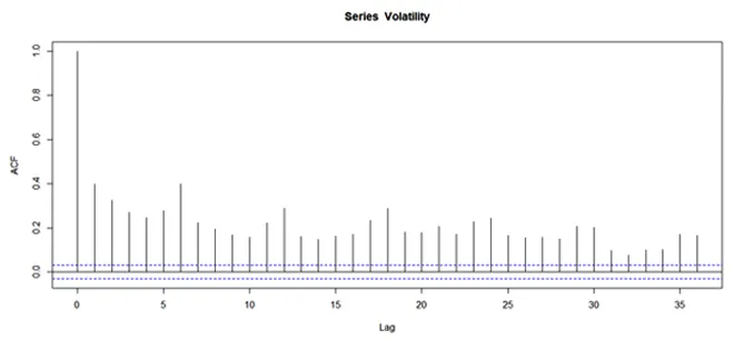
As evident from the results presented in Appendix 1, all the five commodities exhibit mean heterogeneity and some auto-regressive behaviour. The nature of the auto-regressive behaviour is almost the same for all the commodities. A common regression equation is therefore used to check the impact of CTT on the volatility in the futures markets of the chosen commodities. The results of these regression exercises are presented in Table 16.
The trend is for the volatility to increase following the imposition of CTT. This increase is unambiguous in the case of aluminium, copper and gold. In silver, the evidence of an increase in volatility is extremely weak, while in crude oil, an increase in volatility is statistically significant at the 10 percent level of significance.
Table 16: Regression results: Impact of CTT on volatility estimates
| Estimate | Aluminium | Copper | Crude Oil | Gold | Silver |
| β0 | 0.2483*** (0.02567) | 0.2619*** (0.02856) | 0.1638*** (0.02792) | 0.1794*** (0.01869) | 0.2931*** (0.03034) |
| β1 | 0.2349*** (0.01541) | 0.1475*** (0.01482) | 0.1355*** (0.01581) | 0.1632*** (0.01527) | 0.2383*** (0.01535) |
| β2 | 0.1355*** (0.01577) | 0.1019*** (0.01496) | 0.1271*** (0.01585) | 0.1398*** (0.1543) | 0.1209*** (0.01578) |
| β3 | 0.03328* (0.01591) | 0.03653* (0.01502) | 0.05540*** (0.01598) | 0.04776** (0.01559) | 0.04368** (0.0159) |
| β4 | 0.01491 (0.01590) | 0.05700*** (0.01502) | 0.05132** (0.01598) | 0.01837 (0.01559) | 0.007195 (0.01590) |
| β5 | 0.09988*** (0.01574) | 0.06799*** (0.01496) | 0.1136*** (0.01585) | 0.08750*** (0.01543) | 0.05703*** (0.01578) |
| β6 | 0.2435*** (0.01535) | 0.3592*** (0.01481) | 0.3657*** (0.01580) | 0.2729*** (0.01528) | 0.2538*** (0.01535) |
| β7 | -0.00005107*** (0.00001157) | -0.0005296*** (0.00001222) | -0.00001817 (0.00001494) | -0.00003387*** (0.000006743) | -0.00004021** (0.00001491) |
| β8 | 0.06636** (0.02531) | 0.05299* (0.02661) | 0.0584 . (0.03200) | 0.04236* (0.01953) | 0.02449 (0.03387) |
Level of Significance codes: 0 ‘***’ 0.001 ‘**’ 0.01 ‘*’ 0.05 ‘.’ 0.1 ‘ ’ 1 Standard error in parentheses
From Table 17, it is clear that in the case of aluminium and crude oil, price discovery occurs in both markets in the pre-CTT period. However, in both cases, the futures market dominates and therefore leads the spot markets. In the post-CTT period, one would expect the performance of price discovery to take a hit in the futures market. In contrast, the co-efficient of price discovery in the futures markets of these commodities has registered a statistically significant increase whereas the spot markets have experienced a dip in the performance of price discovery in the post-CTT period. As such, the futures markets continue to lead the spot markets in price discovery in the case of aluminium and crude oil.
Expectations of an erosion of the efficiency of the futures markets as regards the function of price discovery after the imposition of the CTT have come true in the case of copper, gold and silver. Prior to the CTT, price discovery occurs in these markets. However, the futures market dominates and therefore leads the spot market in all the three markets.
Following the imposition of CTT, although the spot markets of copper and gold have registered an increase in the performance of price discovery, the increase is not statistically significant. The statistical insignificance of this increase ensures that the futures market continues to dominate the spot market in price discovery despite the decline in the performance of price discovery of the futures market in the case of copper and gold.
In silver, the performance of price discovery of the spot market has registered a statistically significant increase after CTT. However, despite this increase and a dip in the performance of price discovery of the futures market, it is the latter that continues to dominate the function of price discovery as opposed to the spot market.
In summary, the imposition of the CTT may not have adversely affected price discovery in general, but it has had an impact on three of the five commodities chosen for this analysis. This impact of the CTT takes away from any justification for the levy of the tax.
Table 17: Results of the estimation of the Garbade Silber Framework: Impact of
CTT on price discovery
| Estimate | Aluminium | Copper | Crude Oil | Gold | Silver |
| -0.001457838*** (0.000220921) | -0.00438818*** (0.00044486) | -0.002652508*** (0.000257543) | -0.000743220*** (0.000130513) | -0.004107349*** (0.000238487) | |
| 0.000808128*** (0.000240557) | 0.000359970 (0.000249214) | 0.000389421 (0.000347357) | 0.000486166** (0.000167323) | 0.001362607*** (0.000317681) | |
| 0.209600025*** (0.013382535) | 0.96160535*** (0.01482623) | 0.631108472 *** (0.015695642) | 0.697499657*** (0.017255475) | 0.595084179*** (0.014768454) | |
| 0.101199045*** (0.023941706) | -0.24833104*** (0.04611620) | 0.353750023*** (0.025251130) | -0.543072524*** (0.023501227) | -0.277172117*** (0.021331985) | |
| 0.113986842*** (0.014582397) | 0.000249214* (0.008305760) | 0.000347357*** (0.021169268) | 0.047850292* (0.022122895) | 0.073660583*** (0.019672604) | |
| -0.082057338** (0.026091538) | 0.022377170 (0.025834624) | -0.073707180* (0.034057093) | 0.008523532 (0.030130455) | 0.070439715* (0.028415677) |
Level of Significance codes: 0 ‘***’ 0.001 ‘**’ 0.01 ‘*’ 0.05 ‘.’ 0.1 ‘ ’ 1Standard error in parentheses
As Table 18 suggests, in the case of aluminium, the statistically significant increase in the performance of price discovery also translates into increased hedging efficiency. The same is not true for crude oil. In fact, the crude oil futures market registers a decline in hedging efficiency. The decline in the co-efficient of price discovery does not affect the hedging performance of the copper futures market. However, the fall in the performance of price discovery in the gold and silver futures markets has reflected in the decline in their hedging efficiencies. Overall, three of the five commodities investigated for this paper have registered a decline in hedging efficiency on account of the imposition of CTT.
Table 18: Results of the regression estimation and Chow test: Impact of CTT on hedging efficiency
| Estimate | Aluminium | Copper | Crude Oil | Gold | Silver |
| Pre-CTT period | |||||
| 0.00001912 (0.008478) | 0.01499 (0.08383) | 0.15040 (0.36308) | 1.26400 (0.88874) | 2.02491 (3.16576) | |
| 0.7728*** (0.01249) | 0.80907*** (0.03588) | 0.87293*** (0.01208) | 0.84951*** (0.01041) | 0.81100*** (0.01014) | |
| R-squared | 0.6272 | 0.1843 | 0.696 | 0.7503 | 0.743 |
| Post-CTT period | |||||
| 0.006407 (0.009092) | 0.01496 (0.03335) | -0.34155 (0.60461) | 1.89018 (1.33193) | 0.90798 (3.18960) | |
| 0.849555 (0.013774) | 0.77508*** (0.01650) | 0.79234*** (0.01813) | 0.73851*** (0.01142) | 0.71414*** (0.01183) | |
| R-squared | 0.6967 | 0.5711 | 0.6228 | 0.7237 | 0.6977 |
| Chow test p-value | 0.0002206894 | 0.7749527 | 0.0004416195 | 0.0000000000067 | 0.00000001653815 |
Level of Significance codes: 0 ‘***’ 0.001 ‘**’ 0.01 ‘*’ 0.05 ‘.’ 0.1 ‘ ’ 1 Standard error in parentheses
Overall, there has been a decline in the efficiency parameters with the imposition of CTT. Further, when one takes into the consideration the overall decline in turnover of around 66 percent[i] as shown in Table 19, following the analysis of Pavaskar and Ghosh (2008), there should be a consequent decline in government revenue from the commodities markets.[j]
Table 19: Changes in Turnover with Commodity Transaction Tax
| Turnover for all commodities in MCX platform | |
| Year | Total Value (Lacs) |
| 2011 | 1493285202 |
| 2017 | 512604887.5 |
| Change in value in 2017 over 2011 | 980680314.5 |
| %Change in value in 2017 over 2011 | -65.67 |
| Turnover for non-agricultural commodities in MCX platform | |
| Year | Total Value (Lacs) |
| 2011 | 1478693643 |
| 2017 | 500873954.5 |
| Change in value in 2017 over 2011 | 977819688 |
| %Change in value in 2017 over 2011 | -66.12 |
The exercise is replicated using identical assumptions (See Appendix 2) considering the base case of 2011 and estimating the revenue generations from CTT and income taxes in 2011 (prior to CTT imposition) and 2017 to find that there is a net loss to the tax revenue of INR 5562 crores, as shown in Table 20.
Table 20: Turnover and Tax Revenues in 2011 and 2017
| Year | Turnover | Tax revenue generated | Tax revenue generated for Government | Revenue Loss (as compared to 2011) | ||||
| CTT | Brokerages | Commodity Exchanges | Intra-day Traders | Hedgers and Long-term speculators | ||||
| 2011 | 14786936 | 0 | 739.35 | 49.29 | 5914.78 | 2464.51 | 9167.93 | 0 |
| 2017 | 5008740 | 500.874 | 250.44 | 16.70 | 2003.50 | 834.80 | 3606.30 | 5561.63 |
5. Conclusion
This analysis shows that there has been a generic decline in overall market quality in terms of hedging efficiency and price discovery, especially in the context of the liquid commodities. There is no doubt that the CTT has increased the overall cost of hedging. This rise in cost of transaction, whether for hedgers or other market participants, is a retrograde step not only for the commodity exchanges, but for the country’s overall commodity ecosystem. Consequently, the declines in turnover and liquidity due to CTT have affected price discovery function of critical products like gold, silver, and copper, and the hedging efficiency of gold, silver and crude oil. Of these, silver and copper have high utility as industrial inputs. The penchant for gold in India for household purposes and as storage of value is also well-known. The concern is less with crude oil and aluminium: as far as crude oil is concerned, the variety traded in the futures exchange is hardly imported to India, and aluminium has a very low volume to have any substantial effect on physical market trading.
In its pre-Budget memorandum to the Finance Minister, the Commodity Producers’ Association of India sought to make a case that the reduction in CTT would be mutually beneficial, with large revenue gain for the government due to increase in market volumes, creating jobs in the financial sector, and bringing back volumes shifted to overseas countries. They have softened their previous stand of complete removal of the CTT. The CPAI’s idea is that the CTT should be in the range of 0.005- 0.01 percent to boost volumes and treat it as tax paid under Section 88E. However, it is difficult to state from this analysis whether such a scenario is indeed justified. This will require a different type of analysis to understand the critical point of “lafferisation”, i.e., the point in the tax rate axis where revenue loss begins occurring due to volume loss.
This is more so because of the high cost-sensitivity of hedging activities especially in a developing nation like India, where the case of not having such a tax is even more compelling as there is no such “price insurance” mechanism for small producers. A CTT unnecessarily imposes a cost on such small producers and SMEs on insuring themselves against the price risks from increased exposure to international trade and finance. As such, most of the non-agricultural commodities are global commodities whose prices are discovered in international commodity exchanges and through international trading platforms. As India gets more aligned with international trade, the small producers need low-cost risk management platforms to protect themselves against price risks originating from global trading forces. CTT defeats that purpose.
Further, the importance of a risk management platform like derivatives trading arises from two factors: the creation of manufacturing hub as articulated in the government’s Make in India and Self-reliant India visions; and India cannot for long stay away from the forces of globalisation despite its temporary withdrawal from RCEP. India, therefore, needs world-class derivatives exchanges which will provide for the best risk-management practices. It has often been stated that the overall “transaction costs” of doing businesses in India is already very high due to unimplemented labour market reforms, issues with direct taxes and GST compliances, and lack of rationalisations of supply-chains. The CTT has further increased that cost in the form of cost of hedging whose impacts are going to be felt in the entire commodity value-chain within the economy.
While a price discovery function played by an efficient commodity derivatives market would have led to market integration, the CTT’s role in impeding such a function is essentially causing harm to the value chain. As discussed in this paper, even the government is losing out on revenues due to decline in incomes in the commodity derivatives ecosystem because of the CTT. Therefore, there is enough cause to repeal it, as the revenue generated from CTT is far less than the cost that will be borne by the market participants, value-chain stakeholders, and even the government itself due to tax revenue losses.
Appendix 1
Table 1: Regression results for the test of mean heterogeneity for the variable volume traded
| Estimate | Aluminium | Copper | Crude Oil | Gold | Silver |
| α0 | 3048.5589 *** (622.2922) | 63458.703*** (1376.2047) | 4049.9753*** (240.3143) | 40417.8570*** (558.6843) | 1394.23692*** (25.20375) |
| α1 | 10.4846*** (0.2712) | -3.9409*** (0.5989) | 4.0048*** (0.1196) | -7.7180*** (0.2431) | -0.21760*** (0.01095) |
Level of Significance codes: 0 ‘***’ 0.001 ‘**’ 0.01 ‘*’ 0.05 ‘.’ 0.1 ‘ ’ 1 Standard error in parentheses
Table 2: Regression results for the test of mean heterogeneity for the variable turnover
| Estimate | Aluminium | Copper | Crude Oil | Gold | Silver |
| α0 | -33.1502 (784.2185) | 198200*** (5225) | 174000*** (103700) | 543337.495*** (13273.946) | 428007.647*** (14179.626) |
| α1 | 14.0106*** (0.3418) | 2.602 (2.274) | 148.3*** (5.158) | -15.333** (5.777) | -27.228*** (6.162) |
Level of Significance codes: 0 ‘***’ 0.001 ‘**’ 0.01 ‘*’ 0.05 ‘.’ 0.1 ‘ ’ 1 Standard error in parentheses
Table 3: Box-Pierce Q statistics for Volume and Turnover
| Box-Pierce Q Statistic | Aluminium | Copper | Crude Oil | Gold | Silver |
| Volume | 2158.5*** | 1077.8*** | 1275.5*** | 950.04*** | 1167.5*** |
| Turnover | 2414.2*** | 1188.6*** | 1165.1*** | 1142.4*** | 1751.7*** |
Level of Significance codes: 0 ‘***’ 0.001 ‘**’ 0.01 ‘*’ 0.05 ‘.’ 0.1 ‘ ’ 1 Standard error in parentheses
Figure 1: Auto-Correlation Function of the Volume traded for the commodity of Aluminium
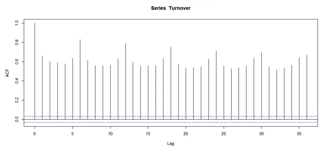
Figure 2: Auto-Correlation Function of the Turnover for the commodity of Aluminium
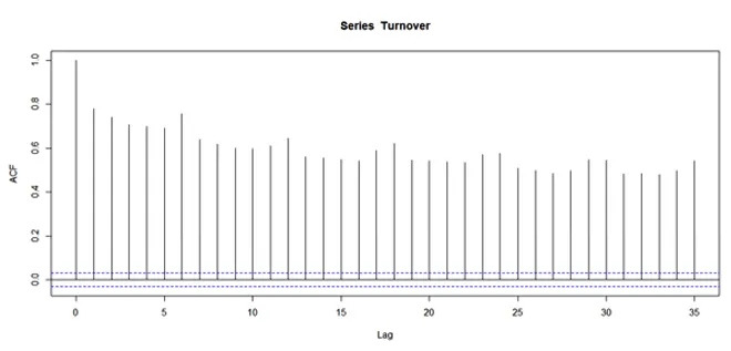
Figure 3: Auto-Correlation Function of the Volume traded for the commodity of Copper
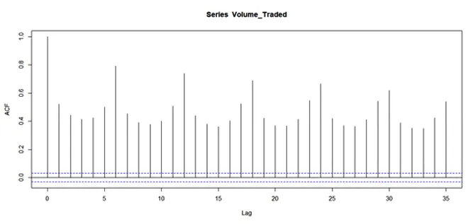
Figure 4: Auto-Correlation Function of the Turnover for the commodity of Copper
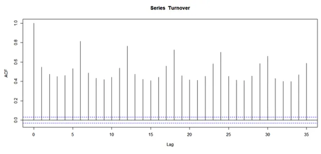
Figure 5: Auto-Correlation Function of the Volume traded for the commodity of Crude Oil
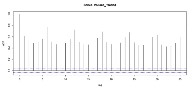
Figure 6: Auto-Correlation Function of the Turnover for the commodity of Crude Oil

Figure 7: Auto-Correlation Function of the Volume traded for the commodity of Gold
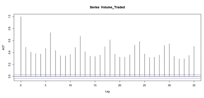
Figure 8: Auto-Correlation Function of the Turnover for the commodity of Gold
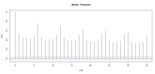
Figure 9: Auto-Correlation Function of the Volume traded for the commodity of Silver
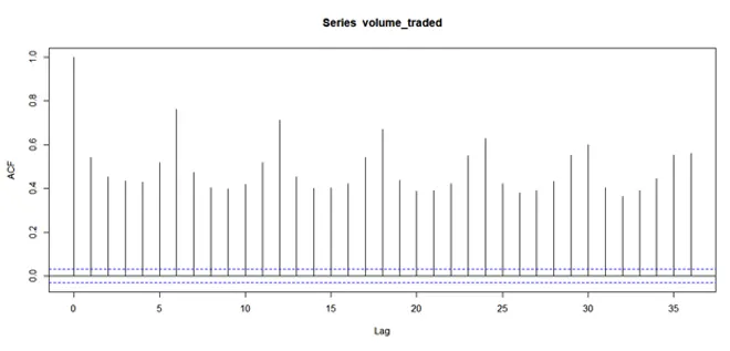
Figure 10: Auto-Correlation Function of the Turnover for the commodity of Silver
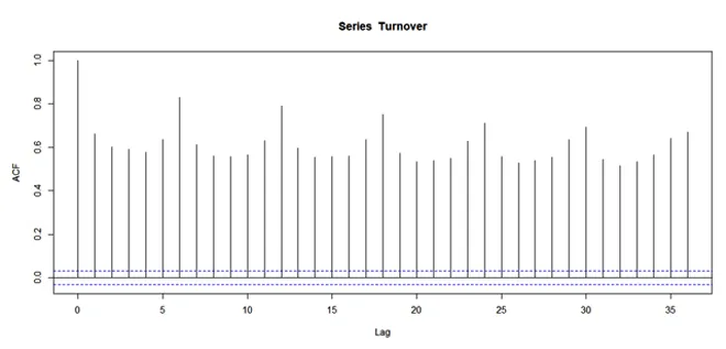
Table 7: Regression results for the test of mean heterogeneity for the Hui-Heubel Ratio:
| Estimate | Aluminium | Copper | Crude Oil | Gold | Silver |
| α0 | 5.951041*** (0.213700) | 1.747*** (0.04830) | 10.960631** (4.209579) | 6.623*** (0.2177) | 0.7992*** (0.15559) |
| α1 | -0.001678*** (0.000094) | -0.00035*** (0.00002102) | -0.002542 (0.002097) | 0.0001422 (0.00009489) | 0.0003495*** (0.00006787) |
Level of Significance codes: 0 ‘***’ 0.001 ‘**’ 0.01 ‘*’ 0.05 ‘.’ 0.1 ‘ ’ 1 Standard error in parentheses
Table 8: Box-Pierce test for the Hui-Heubel Ratio
| Box-Pierce Statistic | Aluminium | Copper | Crude Oil | Gold | Silver |
| For Hui-Heubel Ratio | 65.439*** | 21.048*** | 0.00045212 | 20.735*** | 70.779*** |
Level of Significance codes: 0 ‘***’ 0.001 ‘**’ 0.01 ‘*’ 0.05 ‘.’ 0.1 ‘ ’ 1 Standard error in parentheses
Figure 11: Auto-Correlation Function for the Hui-Heubel Ratio for the commodity of Aluminium
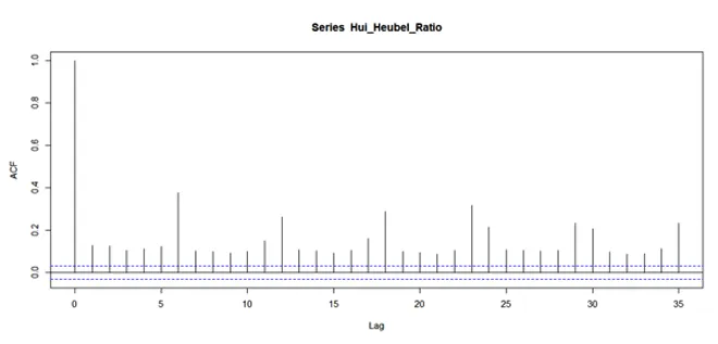
Figure 12: Auto-Correlation Function for the Hui-Heubel Ratio for the commodity of Copper
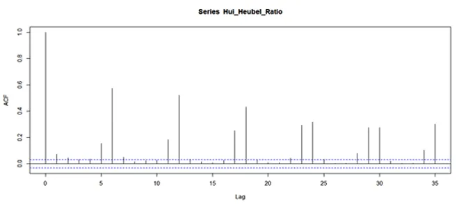
Figure 13: Auto-Correlation Function for the Hui-Heubel Ratio for the commodity of Crude Oil
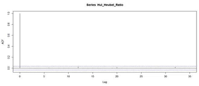
Figure 14: Auto-Correlation Function for the Hui-Heubel Ratio for the commodity of Gold
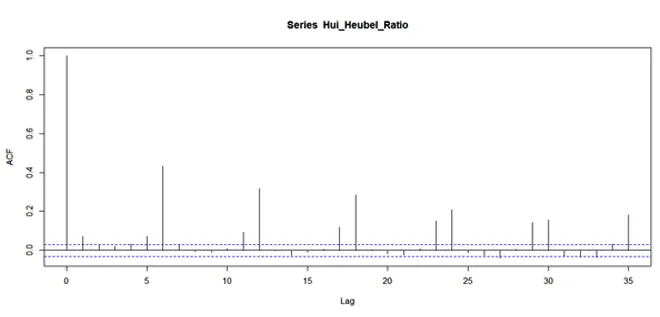
Figure 15: Auto-Correlation Function for the Hui-Heubel Ratio for the commodity of Silver
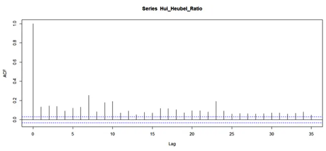
Table 14: Regression results for the test of mean heterogeneity for the volatility estimates:
| Estimate | Aluminium | Copper | Crude Oil | Gold | Silver |
| α0 | 0.9935*** (0.01538) | 1.061*** (0.01596) | 0.9407*** (0.02216) | 0.6150*** (0.01127) | 1.021*** (0.01985) |
| α1 | -0.000125*** (0.000006707) | -0.0001410*** (0.000006948) | 0.00003238** (0.00001103) | -0.00006716*** (0.000004905) | -0.0001106*** (0.000008631) |
Level of Significance codes: 0 ‘***’ 0.001 ‘**’ 0.01 ‘*’ 0.05 ‘.’ 0.1 ‘ ’ 1 Standard error in parentheses
Table 15: Box-Pierce test for the volatility estimates
| Box-Pierce Statistic | Aluminium | Copper | Crude Oil | Gold | Silver |
| For volatility | 954.26*** | 609.64*** | 658.88*** | 505.05*** | 632.62*** |
Level of Significance codes: 0 ‘***’ 0.001 ‘**’ 0.01 ‘*’ 0.05 ‘.’ 0.1 ‘ ’ 1 Standard error in parentheses
Figure 16: Auto-Correlation Function for the volatility estimator for the commodity of Aluminium
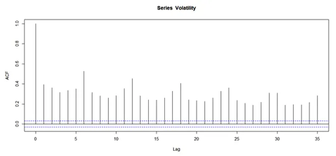
Figure 17: Auto-Correlation Function for the volatility estimator for the commodity of Copper
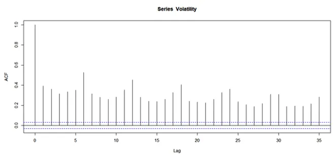
Figure 18: Auto-Correlation Function for the volatility estimator for the commodity of Crude Oil
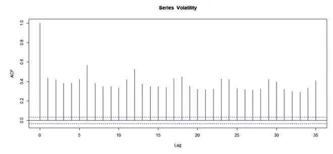
Figure 19: Auto-Correlation Function for the volatility estimator for the commodity of Gold
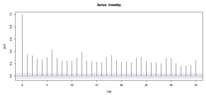
Figure 20: Auto-Correlation Function for the volatility estimator for the commodity of Silver
Appendix 2
Assumptions for estimation of Tax Revenue and Revenue Losses (Based on Pavaskar and Ghosh 2008)
Endnotes
[a] India is the only other country in the world that has a CTT other than Taiwan.
[b]This service of “reference pricing” is popularly known as “price discovery”.
[c] The methodology is motivated by the insights of Aris Spanos and his Probabilistic Reduction Approach. The authors seek to model variables under consideration by specifying a statistical model that captures the systematic statistical information in the data underlying the variables. Graphical techniques and basic statistical testing are utilised. The systematic statistical information is classified into three categories: heterogeneity, dependence, and distribution. Since the sample is large (greater than 3,000 for each variable), it is safe to assume that they are normally distributed by invoking the Central Limit Theorem. As far as heterogeneity and dependence are concerned, the data is examined as mentioned above. Within this econometric framework, the role assigned to the error term is to capture the non-systematic/ random influences/ disturbances in the data. Unlike in the conventional framework in which the objective is to minimise this error, in this case, the paper seeks to render it non-systematic by effectively capturing all the systematic influences present in the data by an appropriate statistical specification.
[d]The choice of commodities was made keeping in mind the need to work with a sample that is representative of the primary product classes in the non-agricultural groups, i.e. base metals, bullion and energy. They are the most heavily traded in terms of value within their product class.
[f]‘Price discovery’is the process of revealing the aggregate information that is sufficient to define an asset’s fundamental price. This fundamental price must be distinguished from the observable price. The first can be deconstructed into the fundamental price and non-systematic/random factors. The latter refers to fluctuations in price such as bid-ask bounce and inventory adjustments.
[g]As compared to the VECM method, the Garbade Silber method is a better tool for this investigation, which seeks to capture the impact of the CTT on price discovery in the long run, rather than the short-run dynamics of the price discovery process.
[i]This is true for decline in overall turnover as also for non-agricultural commodities with around 96-98% of the turnover in MCX being contributed by non-agricultural segment on which CTT is imposed.
[j]Pavaskar and Ghosh talk of a revenue loss in the range of INR 134.8 – 166 billion if the volume declines in the range of 65-75 percent by assuming a case of 0.017 percent of CTT that was initially announced during the Union Budget 2008, but was later withdrawn, and the base case of 2007.
[1] Press Trust of India, “Transaction tax on non-agri futures trade introduced,” Business Standard, February 28, 2013.
[2] Madhoo Pavaskar, ‘Commodity Exchanges Are Not Stock Exchanges’, Economic & Political Weekly, Vol XXXIX, No 48, November 27-December 3 (2004); Madhoo Pavaskar & Nilanjan Ghosh, “Commodity Transaction Tax: A Recipe for Disaster”, Economic and Political Weekly, Vol. 43, No. 39(2008).
[3] Sanjay Sehgal and Tarunika Jain Agrawal, “Impact of Commodity Transaction Tax on Market Liquidity, Volatility, and Government Revenues: An Empirical Study for India,” Vikalpa: The Journal for Decision Makers 44, no. 1(2019).
[4] Pavaskar and Ghosh, “Commodity Transaction Tax: A Recipe for Disaster”
[5] Pavaskar and Ghosh, “Commodity Transaction Tax: A Recipe for Disaster”
[6] Narinder Wadhwa, “Budget 2020: These 2 reforms by FM Nirmala Sitharaman can boost commodity market participation,” Financial Express, January 10, 2020.
[7] Press Trust of India, “CPAI proposes govt to rationalise CTT to boost volumes,” The Economic Times, January 13, 2021.
[8]Pavaskar and Ghosh, “Commodity Transaction Tax: A Recipe for Disaster,” Pravakar Sahoo and Rajiv Kumar, “Impact of Proposed Commodity Transaction Tax on Futures Trading in India,” ICRIER Working Paper No. 216, 2008.
[9] Nilanjan Ghosh,” Issues and Concerns of Commodity Derivative Markets in India: An Agenda for Research,” Commodity Vision, Volume3, Issue no.4 (2009), 8-19.
[10] Isabel Figuerola-Ferretti and Jesús Gonzalo. Modelling and measuring price discovery in commodity markets. Journal of Econometrics 158(2010).
[11] Pantisa Pavabutr & Piyamas Chaihetphon, “Price discovery in the Indian gold futures market,” Journal of Economics and Finance. 34(2009).
[12] Pavaskar and Ghosh, “Commodity Transaction Tax: A Recipe for Disaster”.
[13] Pavaskar and Ghosh, “Commodity Transaction Tax: A Recipe for Disaster”.
[14] Sahoo and Kumar, “Impact of Proposed Commodity Transaction Tax on Futures Trading in India”
[15] Nilanjan Ghosh, “Role of Thin Commodity Futures Markets in Physical Markets Price Making: An Analysis of Wheat Futures in India in the Post-Ban Era”, Independent Business Review, Volume 3, Issue no.2 (2010).
[16] C. A. Carter, “Arbitrage opportunities between Thin and Liquid Futures Markets”, Journal of Futures Markets, Volume 9, No. 4 (1989).
[17] Charles M. Seeger, “India’s Commodity Transaction Tax: Economic Consequences and International lesson learned,” Financial Markets International, Inc, 12(2013).
[18] Pavaskar and Ghosh, “Commodity Transaction Tax: A Recipe for Disaster”
[19]Sehgal and Agrawal, “Impact of Commodity Transaction Tax on Market Liquidity, Volatility, and Government Revenues: An Empirical Study for India.”
[20] Pavaskar and Ghosh, “Commodity Transaction Tax: A Recipe for Disaster”.
[21] Sehgal and Agrawal, “Impact of Commodity Transaction Tax on Market Liquidity, Volatility, and Government Revenues: An Empirical Study for India.”
[22] Pankaj Sinha and Kritika Mathur, “Securities Transaction Tax and the Stock Market: An Indian Experience,” Finance India, Volume 28, No.2 (2014).
[23] Sehgal and Agrawal, “Impact of Commodity Transaction Tax on Market Liquidity, Volatility, and Government Revenues: An Empirical Study for India.”
[24] Sahoo and Kumar, “Impact of Proposed Commodity Transaction Tax on Futures Trading in India;” Sehgal and Agrawal, “Impact of Commodity Transaction Tax on Market Liquidity, Volatility, and Government Revenues: An Empirical Study for India;” Robin K. Chou and George H. K. Wang, “Transaction Tax and Market Quality of the Taiwan Stock Index Futures,” Journal of Futures Markets Volume 26, No. 12 (2006).
[25] Sinha and Mathur, “Securities Transaction Tax and the Stock Market: An Indian Experience”
[26] Sahoo and Kumar, “Impact of Proposed Commodity Transaction Tax on Futures Trading in India”
[27] Sahoo and Kumar, “Impact of Proposed Commodity Transaction Tax on Futures Trading in India”
[28] Sehgal and Agrawal, “Impact of Commodity Transaction Tax on Market Liquidity, Volatility, and Government Revenues: An Empirical Study for India.”
[29] Pankaj Sinha and Kritika Mathur, “Impact of commodities transaction tax on Indian commodity futures,” MPRA Working Paper No. 63677 (2015).
[30] Sehgal and Agrawal, “Impact of Commodity Transaction Tax on Market Liquidity, Volatility, and Government Revenues: An Empirical Study for India.”
[31] Sehgal and Agrawal, “Impact of Commodity Transaction Tax on Market Liquidity, Volatility, and Government Revenues: An Empirical Study for India.”
[32] Sinha and Mathur, “Securities Transaction Tax and the Stock Market: An Indian Experience;”
[33] Yongyang Su & Lan Zheng, “The Impact of Securities Transaction Taxes on the Chinese Stock Market. Emerging Markets Finance and Trade.” Volume 47 (2011).
[34] Sahoo and Kumar, “Impact of Proposed Commodity Transaction Tax on Futures Trading in India”
[35] Sehgal and Agrawal, “Impact of Commodity Transaction Tax on Market Liquidity, Volatility, and Government Revenues: An Empirical Study for India.”
[36] Saon Ray, & Neha Malik, “The impact of transaction taxes on commodity derivatives trading in India,” ICRIER Working Paper No. 272 (2014).
[37] Sinha and Mathur, “Impact of commodities transaction tax on Indian commodity futures”
[38]Diganta Mukherjee, “Economic impact of commodity transaction tax on futures contracts,” Prajnan, Volume 46, No.2, (2017).
[39] Velmurugan Shanmugan and Rinku Champramary, “CTT Infuses Inefficiency into Gold Futures Trading: An Empirical Analysis,” SSRN Electronic Journal (2016).
[40] Sehgal and Agrawal, “Impact of Commodity Transaction Tax on Market Liquidity, Volatility, and Government Revenues: An Empirical Study for India.”
[41] Aris Spanos, Probability Theory and Statistical Inference: Econometric Modeling with Observational Data (Cambridge: Cambridge University Press, 1999).
[42] Spanos, Probability Theory and Statistical Inference: Econometric Modeling with Observational Data
[43] Sehgal and Agrawal, “Impact of Commodity Transaction Tax on Market Liquidity, Volatility, and Government Revenues: An Empirical Study for India.”
[44] Chou and Wang, “Transaction Tax and Market Quality of the Taiwan Stock Index Futures.”
[45] M. T. Raju and Kiran Karande, “Price Discovery and Volatility on NSE Futures Market,” SEBI Working Paper No. 7 (2003).
[46] Erik Theissen, “Price discovery in spot and futures markets: A reconsideration,” European Journal of Finance, Volume 18, No 10 (2012).
[47] Susan Thomas & Kiran Karande, “Price Discovery Across Multiple Spot and Futures Markets,” Proceedings of Capital Market Conference (2002).
[48] Thomas & Karande, “Price Discovery Across Multiple Spot and Futures Markets”
[49] “Hedging Efficiency: A Comparative Assessment of MCX vis-à-vis Global Exchanges,” MCX Occasional Paper Series No.2/2013 (2013).
[50] “Hedging Efficiency: A Comparative Assessment of MCX vis-à-vis Global Exchanges,” MCX Occasional Paper Series No.2/2013
The views expressed above belong to the author(s). ORF research and analyses now available on Telegram! Click here to access our curated content — blogs, longforms and interviews.

Dr Nilanjan Ghosh is Vice President – Development Studies at the Observer Research Foundation (ORF) in India, and is also in charge of the Foundation’s ...
Read More +
Renita DSouza is a PhD in Economics and was a Fellow at Observer Research Foundation Mumbai under the Inclusive Growth and SDGs programme. Her research ...
Read More +