Introduction

India belongs to the category of water-stressed nations, and water scarcity is a painful reality in many parts, especially during the dry seasons. The renewable internal freshwater resources per capita, as of 2017, was as low as 1,080 m³ for India against the global average of 5,732 m³.^[a],[1] Unless current patterns are reversed, India will soon become a water-scarce country.^[b] Despite being home to 16-17 percent of the world’s population, India accounts for only four percent of global freshwater resources.^[2]

The demand for water in India is driven by a rapidly increasing population and their demand for food, as well as the accompanying economic growth and development. At the same time, supply is constrained owing to worsening water pollution, frequent droughts as an impact of climate change, poor water resource management systems that result in water overuse and thus, depletion in groundwater tables.  The problems are aggravated by global warming, which is poised to create severe stress on future water availability in the sub-continent.

According to latest assessments, annual precipitation recorded in India stands at about 3,880 BCM (Billion Cubic Metre). On account of topographic, hydrological, and other constraints, the volume of utilisable water is 1,122 BCM—690 BCM of surface water and 432 BCM of total annual groundwater recharge. However, lack of appropriate water management techniques prevents the optimal utilisation of this utilisable water. For example, due to low and erratic rainfall patterns in areas experiencing chronic water stress, water harvesting structures fail to contain the minimum volume of water necessary for making water conservation strategies feasible.^[3]

India ranks second globally in farm production and output,^[4] underscoring the critical role of water in the country’s agriculture sector. Globally, India stands first in milk production, second in dry fruits, third in fish output, fourth in eggs, and fifth in poultry production; it is also the largest producer of wheat.^[5] Around 70 percent of India’s population are employed in agriculture, exerting further pressure on water resources.^[6]

A straightforward definition of ‘water-use efficiency’ in agriculture is crop yield per unit of water consumed or financial returns on investment made in water supply infrastructure. In this respect, India has very low water-use efficiency. Given that agriculture dominates water use in India, the agricultural practices of water management bear significantly upon the strategy for coping with the ongoing water crisis in the country. More specifically, attention needs to be drawn to the over-exploitation of groundwater resources and inefficient irrigation systems. Unless water-use efficiency is addressed effectively in the agricultural sector, other water-management practices will fall short of coping with water stress.

Around 55 percent of India’s arable land rely heavily on monsoons.^[7] Therefore, the occurrence of droughts has a massive impact on water availability, and consequently, on agricultural productivity and output. There has been a significant rise in the frequency of droughts in the past three decades, and experts project that this pattern will only worsen from now up till 2049.^[8] Some 26 episodes of drought occurred from 1870 to 2018 in India. The most recent drought, which occurred during 2015-2018, was the longest; although it was less severe than other droughts in the past, it brought disaster to the agriculture sector and underlined the threats of water security.^[9] To compensate for water shortage that result from droughts, groundwater resources are relied upon; this in turn increases the stress on these resources.

Can greater water-use efficiency in agriculture ease the pressure on India’s water resources? This paper investigates the use of water for different crops, and explores a shift to more water-efficient alternatives. The rest of the paper culls insights from current literature; outlines the methodology used by the authors to estimate the marginal product of water in terms of crop output and nutrients; describes the findings of the analysis; contemplates the implications on crop performance in relation to water use efficiency in nutrient production; outlines the policy implications; and argues in favour of Integrated Water Resource Management (IWRM) in managing water use in agriculture. 

Water for Agriculture: The Indian Case

The irrigation sector accounts for 80 percent of total water consumed in India.^[10] Groundwater irrigation accounts for 70 percent of both total irrigated area and agricultural output in the country.^[11] India is home to the largest number of irrigation wells (around 30 million), and pumps twice the water as that of the United States (US) and six times that of the European Union (EU).^[12] These reserves are being utilised in an unsustainable manner because of various reasons: distorted subsidies including free electricity for pumping groundwater, concessional pricing of water pumps, input subsidies that further incentivise intensive cultivation and, in turn, the exploitation of groundwater reserves.  Distorted water pricing is also responsible for overextraction of India’s groundwater, which is depleting at a rate of 0.3 metres annually.^[13] Nearly one-sixth of India’s groundwater assessments units are categorised as ‘over-exploited’, while 15.2 percent are in ‘semi-critical’ and 3.9 percent are in ‘critical state’.^[14]

Given that the irrigation sector is a user of massive amounts of water, it is necessary to translate the ‘per drop more crop’ mantra to reality. This could yield the best possible outcome in ensuring food security while achieving appreciable water savings.

The heavy reliance on water as an agricultural input in India is explained by the composition of crop production in the country. Rice, wheat and sugarcane represent 90 percent of India’s crop production.^[15] It is known that these crops are all heavy water users. While rice, wheat, cotton and sugarcane represent 46 percent of the Gross Cropped Area, their production accounts for 65 percent of the Gross Irrigated Area.

Minimum Support Prices (MSP) has a direct link to Public Distribution System (PDS) availed by 67 percent of the country’s population. Under the PDS, food grains are provided to the poor at subsidised rates through fair price shops. MSP incentivises farmers to grow crops which are procured by the government.  As wheat and rice are major food grains provided under the PDS, the focus of procurement is on these crops.  This skews the production of crops in favour of wheat and paddy (particularly in states where procurement levels are high) and does not offer an incentive for farmers to produce other items such as pulses.  Further, this puts pressure on the water table as these crops are water-intensive.^[16]

Perverse incentives in the form of MSP have led to the trend of cultivating these water-intensive crops even in highly water-stressed regions by applying 100 percent irrigation; this puts great pressure on groundwater resources. For example, despite being under severe water stress, Punjab and Maharashtra cultivate rice and sugarcane, relying completely on irrigation. In Punjab, this has translated into 166 percent of groundwater extraction. These water-intensive crops are grown in areas where such cultivation demands a large dependence on irrigation but the irrigation water productivity is really low.^[17] To what extent these water guzzlers are relied upon for food security has implications for improving water-use efficiency and in turn, water productivity,^[c] in the context of crop cultivation in particular and the agricultural sector, overall.

The government of India recognises the urgency of launching initiatives that are needed to mitigate overextraction and overuse of water and to promote sustainable management of water resources driven by water use efficiency and increased water productivity. In May 2019, the Ministry of Jal Shakti was created to consolidate efforts directed at sustainable water management. The ministry has envisioned schemes to enhance irrigation efficiency and outreach, and optimal utilisation of water resources through innovative measures. The programmes include:

i.) Pradhan Mantri Krishi Sinchayee Yojana (PMKSY)^[18]

The scheme was launched in 2015 to extend the coverage of protective irrigation across all agricultural farms in India; enhance farm water use efficiency; promote the adoption of, and improve investments in precision agriculture and other water-saving technologies; augment the recharge of aquifers; and encourage sustainable water conservation.

ii.) Atul Bhujal Yojana^[19]

The scheme focuses on sustainable groundwater management, with an emphasis on community participation and demand-side interventions. It was launched in 2020 in 8,353 water-stressed Gram Panchayats of Haryana, Gujarat, Karnataka, Madhya Pradesh, Maharashtra, Rajasthan, and Uttar Pradesh.

iii.) Micro Irrigation Fund, NABARD^[20]

With a corpus of INR 5000 crore, the fund is designed to support initiatives of state governments for mobilising finance for expanding coverage under micro-irrigation and encouraging its adoption beyond PMKSY.

iv.) Sahi Fasal Campaign, National Water Mission^[21]

This campaign was launched to encourage farmers, especially in water-stressed areas, to migrate from the cultivation of water-intensive crops to those less so, and which are not only economically remunerative but also rich in nutrition. It also aims to ensure that cultivation is undertaken based on the agro-climatic-hydro characteristics of the region. A primary strategy is raising awareness among farmers on issues such as appropriate crops, micro-irrigation, and soil moisture conservation. The mission also seeks to assist policymakers in appropriate pricing of inputs such as water and electricity, provision of adequate storage facilities for these alternative crops, and enhance procurement and expand markets for them.

Review of Literature

There is no dearth in literature on water-use-efficiency estimates across crops. These studies, however, are sparse in India, or even in South Asia. In more recent years, however, such studies have started emerging in the context of the countries in the subcontinent.

At a conceptual level, Morrison et al. (2007)^[22] approached the issue of crop water use through the physiological lens and investigated the underlying relationships between carbon uptake, growth, and water loss. For their part, Kaur et al (2010)^[23] devised a linear programming model to determine the optimal cropping patterns in the state of Punjab. Waraich et al. (2011),^[24] meanwhile, presented an elaborate discussion on how plant nutrients enhance WUE and productivity in crop plants. Their study identified the adverse effects of limited water supply and drought conditions in the form of destruction of physiological processes on plant growth and development.

Descheemaeker et al. (2013)^[25] are motivated by the hypothesis that enhancing water productivity is crucial for effective water management underlying sustainable agriculture, food security, and well-functioning ecosystems. Their study explored the difficulties involved in, and solutions for boosting water productivity in a sustainable and equitable manner. Meanwhile, Dhawan (2017)^[26] attributed water-shortage in India to poor water resource management, and implicitly connected food security with the need for infrastructure expansion and improved resource utilisation. Sharma et al. (2018)^[27] examined whether existing cropping patterns in India align with the distribution of water resources across regions. The study identified strategic policy options such as: (a) appropriate pricing, improved quality and assured supply of water and electricity in agriculture; (b) better and assured procurement policy regime in states with high IWP; (c) direct benefit transfer of input subsidies; (d) market determination of prices; and (e) adoption of best practices relating to improved water management. The second-best solution to pricing reforms would be the rationing of irrigation water and power supply.

Zahoor et al. (2019),^[28] for their part, aimed at providing direction to the policy of water resource management to mitigate increasing water risks adversely affecting agricultural production, trade, and food security. Otárola et al. (2020)^[29] simulated WUE of crops under different irrigation strategies in the Central Valley of Chile. The simulation exercise provided estimates of the impact of a given or in-use irrigation method and heuristics about better irrigation practices.

Shukla et al. (2021)^[30] argued that an ecosystem for increasing water-use efficiency in agriculture should be composed of several components including technology, cropping patterns, governance institutions, and policy frameworks. Mehta and Maggo (2021),^[31] building on the 2014 report published by World Business Council for Sustainable Development (WBCSD), highlighted the utility of these co-optimising solutions in the specific context that places special emphasis on water and agriculture. The study by Kumar et al. (2021), meanwhile,^[32]  estimated the water use and water productivity of different crops grown in an intensively groundwater irrigated watershed.

One study that has addressed the same issue as the present paper was that by Davis et al. (2018):^[33] how to use water more efficiently while enhancing nutrient production. Using the concept of water footprint, it explored the shifts in cropping patterns from the dominant wheat-rice system to alternative crops including maize, jowar, ragi, and bajra. However, the present paper differs from that of Davis et al. in how it measures water productivity. Instead of water footprint, this analysis uses the marginal product of water to reflect crop water productivity. The marginal product of water quantifies the gains in terms of crop output and nutrient production that follow from applying an additional megalitre of water to cultivation of the concerned crop. Gains in nutrient production and water savings from replacing rice with alternative cereals are computed by applying a simple investigative analysis based on the marginal products of water in the context of different crops.

This review of literature indicates that existing research on improving water use efficiency in agriculture explicates the various ways in which the notion of water use efficiency can be approached, and offers recommendations in exploring the opportunities that thereby follow. There has been little research dealing with nutritional security and water security in an integrated framework. This paper seeks to bridge the gap. 

Methodology

The Cobb-Douglas Framework

Assuming that India’s agricultural production behaves in accordance with a Cobb-Douglas function whose parameters have remained constant across the period of study, this exposition quantifies the marginal product of water measured in terms of nutrients contained in a given crop. More specifically, the measure informs us about the nutritional gains accrued by applying an additional unit of water to the cultivation of the concerned crop. The log-linear form of the Cobb-Douglas production function is estimated. While the water input required for the production of each crop under study will be computed, the crop yield will act as a proxy for the total factor productivity and the intensive use of other inputs involved in crop cultivation. The crop water input captures land input (and its extensification) and the application of water required for crop cultivation to this land.^[34] In the log linear regression of the Cobb Douglas function, the crop production is regressed on crop yield and water input.

An exposition of the Cobb-Douglas production function is given below through the mathematical framework. The framework adequately explains how marginal product of water for a crop captures land’s marginal product.

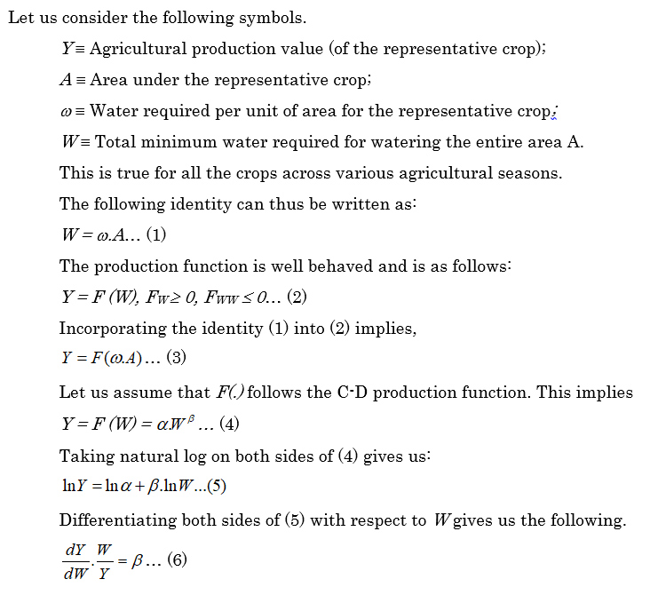
The left-hand-side of (6) is nothing but the elasticity of production with respect to water, or in other words, the percentage change of production if water input changes by a percent. The equation therefore shows that β is the elasticity of production with respect to water.

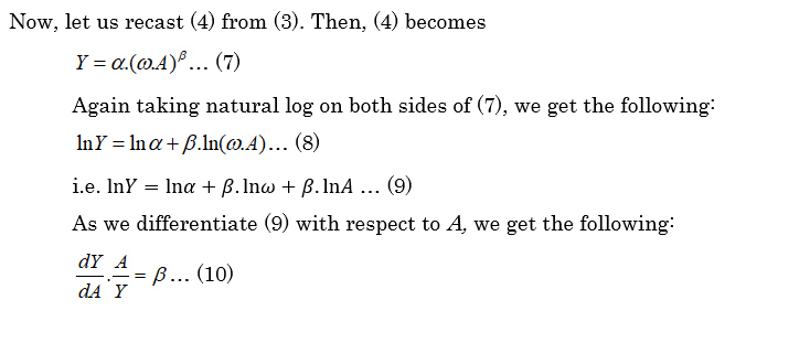
The assumption here is that and do not vary with A. The left-hand-side of (10) is nothing but the elasticity of production with respect to area. One may also note the equivalence of the left-hand-side of (6) and (10). Therefore, the exercise clearly shows that the elasticity of water use and land with respect to production are the same in the case of the specific crop under consideration. In other words, the productive efficiency of water reflects on the productive efficiency of land. The framework therefore automatically assumes the diminishing marginal product of land through the diminishing marginal product of water.

The econometric framework and estimation process

Once the regression determines the water elasticity of crop output, the next step is to determine the average product of water in terms of crop output measured in kilograms. This value is given as the average product of water of the latest year in the study period.^[d] As can be made out from (6), multiplying this average product with the water elasticity of crop output yields the marginal product in terms of crop output. Based on the nutritional information of various crops, the marginal product of water in terms of nutrients is determined. This figure reflects the nutritional gains acquired by applying an additional input of water to the production of a crop. In this context, this paper takes into consideration the annual water use for the crops, as for the marginal product estimation seasonality is irrelevant. All the crops taken into consideration have their irrigated acreages annually, while some of them are largely grown during monsoons. Therefore, in line with previous studies,^[35] this paper does not assume that there is a difference in the marginal product of irrigation waters and the monsoon waters. At an annual scale, such a difference does not make sense. For that purpose, the assumption is that there is no difference in the marginal contribution of rainwater and irrigation water, implying that the source of water is irrelevant.

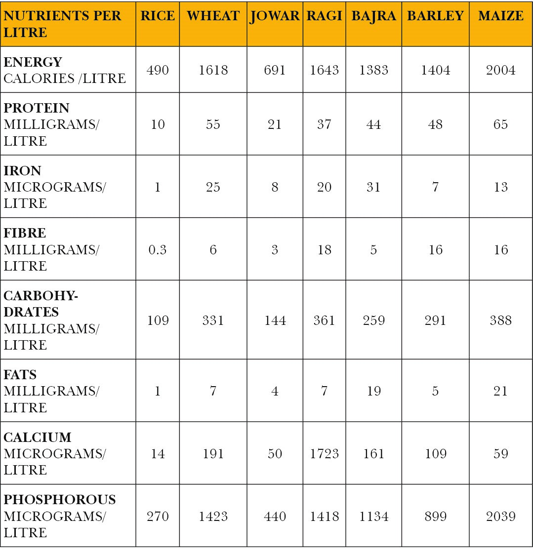
For our analysis, we have taken into consideration the following crops: rice, wheat, jowar, ragi (finger millet), maize, bajra (pearl millet) and barley. The nutrients of interest include calories, protein, iron, fibre, carbohydrates, fat, calcium, and phosphorous. The period under study is 1967-2019.

We present the steps in the methodology used to compute the marginal product of water in terms of crop nutrient value as regards the above-mentioned crops. 

Step one: Calculation of the crop water requirement for the period under study (1967 -2019):

The Blaney-Criddle (BC) approach has been deployed to calculate annual water requirement of each crop across its growing season in the study period. Since the only available dataset for the period under study was that of monthly temperature, the BC approach which relies only on temperature was used for the purpose. The BC approach provides rough estimates and is susceptible to biased estimation in extreme conditions. Since the present paper is a comparative analysis across various crops, the fact that that the BC approach is consistently applied in estimation of water requirement across all crops renders the problem of biased estimation as an unimportant one. The reference evapotranspiration, and the crop factor used to calculate the annual crop water requirements are those recommended by the Food and Agriculture Organisation (FAO). The calculated values have been adjusted based on the information on India-specific crop water requirements. The details of this approach are given in the Appendix. 

Step two: Calculation of the water input involved in the production of each crop under cultivation.

The input of water used in the production of each crop for every year from 1967 to 2019 is obtained as the product of the India-adjusted total annual crop water requirement and the area (hectares) under cultivation. To obtain the water input in terms of megalitres, the above-mentioned product is divided by 100. 

Step three: Identification of components of non-stationarity contained in stochastic processes underlying variables under investigation.

The objective is to obtain the marginal product of water in terms of crop calorific value. To that end, the first step is to obtain the marginal product of water as additional crop production following from applying an additional unit of water. The next step is to determine the additional nutrients that would accrue from applying an additional unit of water to the production of a given crop. In this step, the additional crop production entailed by the application of an additional unit of water is simply multiplied by the units of nutrients contained in single unit of a given crop.

The investigation is in search of a regression model that exhaustively explains all of the variation in the prospective regressand. The variable under consideration as the regressand is the logarithmic transformation of the production of each crop over the period under study 1967-2019. The logarithmic transformation of the crop yield and the crop water input for are the prospective regressors. The lagged values of logarithmic transformations of the crop production, the yield and the water input will also be considered as prospective regressors.

First, the investigation examines the pattern of non-stationarity of the main variables—i.e., the crop production, the crop yield, and the crop water input. To identify the components of non-stationarity, the Augmented Dickey-Fuller test (ADF) with a drift and a linear trend is applied in combination with regression-based tests. It has been observed that the ADF test may not always be capable of detecting multiple components of non-stationarity and past information, namely unit root and linear trend. In many instances, it might either detect the unit root or the linear trend, but not both. In the current investigation, quadratic trends have also been detected. Therefore, a combination of the ADF test and the regression-based test.

Confirmatory regression-based tests are exploratory in nature. In this paper, unit root, linear trend and quadratic trend are the components of non-stationarity which have been detected. Iterations of regression are run with each new iteration including a different element or a combination of elements which capture non-stationarity and memory. Regressions are run till all combinations of non-stationarity and memory components are exhausted, in this case, varying combinations of the autoregressive term, linear trend and quadratic trend are included in identifying patterns of non-stationarity.

While the information provided by the ADF test may help in extracting elements of non-stationarity and render the process stationary, by identifying other sources of non-stationarity apart from those done by the ADF test, the regression-based tests provide necessary information which can be used to alternatively model the non-stationarity. Why this is helpful has been explained in the latter sections and the appendix.  An illustration of the same is presented in the appendix in the context of a single crop, namely wheat. An exhaustive explication of the exercise of detecting the components of non-stationarity in the context of the remaining crops has been excluded for lack of space.

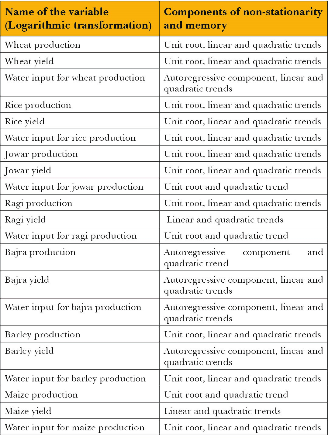
Employing the same procedure used to identify the components of non-stationarity contained in the stochastic processes underlying the logarithmic transformations of wheat production, wheat yield and water input for wheat production as explicated in the appendix, components of non-stationarity and memory have been uncovered for other stochastic processes as well.  Table 1 enlists the components of non-stationarity detected in each of the stochastic processes underlying variables under study: 

Table 1: Components of non-stationarity and memory in stochastic processes

Step four: Creation of two types of stationary variables: (i) Stationary variables which represent current or new information associated with the variable and (ii) Stationary variables which contain past/lagged information in the form of autoregressive component of the variables.

Two sets of variables are intended to be included into the main regression and hence, in creating stationary variables, two approaches have been adopted: The first approach seeks to create stationary variables which contain current or new information by deducting the past information that comprises the observation. As far as the trend is concerned, there are two components to it, one of which corresponds to the past and the other to the current information.

Depending upon the components of non-stationarity, the process of differencing/de-memorising in the case of unit root and detrending in the case of trends is used. In the presence of both unit root and trends, both the processes are applied.

After deducting the non-stationary components, the i^th observation should contain the information associated with the i^th year. More specifically, the i^th observation will contain the i^th error term along with the recurring constant term and the regression coefficient of the trend terms which represent current/new information associated with the i^th year.

In the second approach to creating stationary variables, the lagged values of the variables under investigation are considered. In this approach, the lagged values are simply detrended to retain the autoregressive and error components comprising the observation. In this case, the stationary variables contain only the past information as represented by the autoregressive and the error terms. As mentioned above, while detecting components of non-stationarity, the ADF test results were complemented with exploratory regression-based tests. The information provided by these tests suggest an alternative way of modelling non-stationarity apart from the unit root. This allowed to create a new variable which while capturing the lagged autoregressive component could be stationary at the same time due to a simple detrending process.

To be sure that the newly created variables are indeed stationary, stationarity tests were run. Results of ADF tests for each of the newly created current variables have been reported in the appendix. 

Step five: Running of the regression which includes the stationary variables created in the previous step.

Given that the newly created variables are indeed stationary, the main regression model can now be run which includes these newly created variables.

The regressand of the main regression is the stationary variable on logarithm of crop production which is composed of the current or new information. The regressors include the stationary variables comprising current information on logarithm of crop yield and crop water input. The regressors also include stationary variables comprising lagged values on logarithms of crop production, crop yield and crop water input. However, the regressors comprising current information on crop yield and crop water input turn out to be statistically significant across all crops. However, the same is not true for the regressors comprising lagged information. Not all of these regressors turn out to be statistically significant in all cases. Hence their inclusion in the main regression model depends upon whether they are statistically significant or not.

The basic structure of the main regression model for each crop is essentially the same. It is as follows:

P_t = α+β₁Y_t + β₂WI_t + β₃P_t-1+β₄Y_t-1 + β₅WI_t-1 + e_t                                                                                                (1)

Where:

P_t: Stationary version which represents the current/new information contained in the production variable of a given crop

Y_t: Stationary version which represents the current/new information contained in yield variable of a given crop

WI_t: Stationary version which represents the current/new information contained in the water input variable for production of a given crop

P_t-1: Stationary version which represents the lagged/past information contained in production variable of a given crop

Y_t-1: Stationary version which represents the lagged/past information contained in yield variable of a given crop

WI_t-1: Stationary version which represents the lagged/past information contained in the water input variable for production of a given crop

The regression coefficient β₂ represents the water elasticity of crop output which then multiplied by the average product of water to arrive at the marginal product of water in term of crop output (in kgs). The rest of the calculation procedure has already been explicated at the beginning of the methodology section.

Results and Discussion

Wheat

For wheat, the regression co-efficient on the variable WI_t-1 is statistically insignificant.

The results of the estimation are as follows: 

Table 2: Summary output for the main regression for wheat

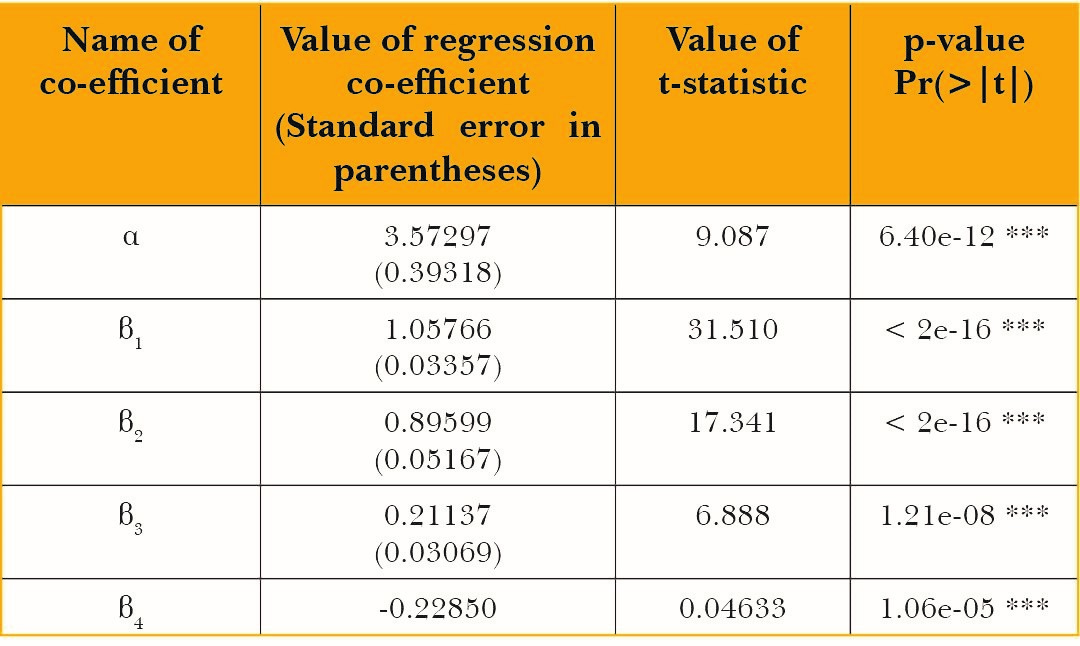
Signif. codes:  0 ‘***’ 0.001 ‘**’ 0.01 ‘*’ 0.05 ‘.’ 0.1 ‘ ’ 1
Adjusted R² of the regression: 0.964

The diagnostic tests run on the residuals of the regression exhibit no autocorrelation, homoskedasticity and normality of residuals. Results are presented in the appendix.

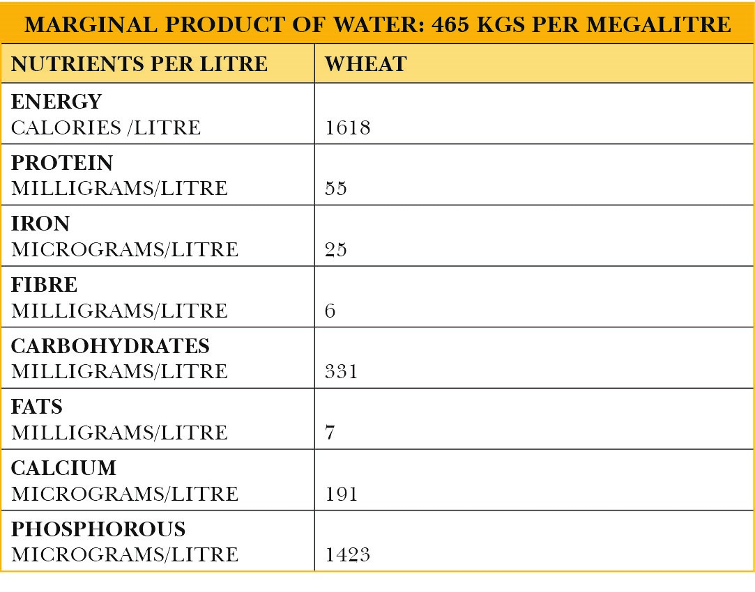
The regression co-efficient β₂ is the production elasticity of water input which equals 0.89. Multiplying this by the average product of water gives the marginal product of water which is equal to 465 kgs per megalitre of water. The marginal product in terms of the nutrients contained in wheat is as follows: 

Table 3: Marginal product of water in terms of terms of output as well as nutritional content of wheat

1.1 Rice

For rice, the regression coefficient of WI_t-1is statistically insignificant. 

Table 4: Summary output for the main regression for rice

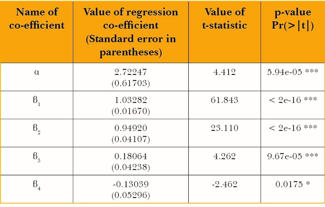
Signif. codes:  0 ‘***’ 0.001 ‘**’ 0.01 ‘*’ 0.05 ‘.’ 0.1 ‘ ’ 1
Adjusted R² of the regression: 0.9942

The diagnostic tests run on the residuals of the regression exhibit no autocorrelation, homoskedasticity and normality of residuals. Results are presented in the appendix.

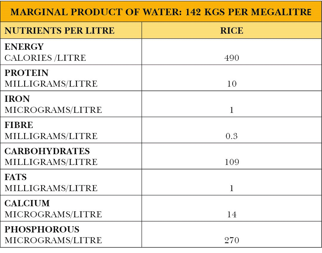
The regression co-efficient β₂is the production elasticity of water input which equals 0.95. Multiplying this by the average product of water gives the marginal product of water which is equal to 142 kgs per megalitre of water. The marginal product in terms of nutrients contained in rice is as follows: 

Table 5: Marginal product of water in terms of terms of output as well as nutritional content of rice 

Jowar

For Jowar, the regression coefficient of WI_t-1is statistically insignificant. 

Table 6: Summary output for the main regression for jowar

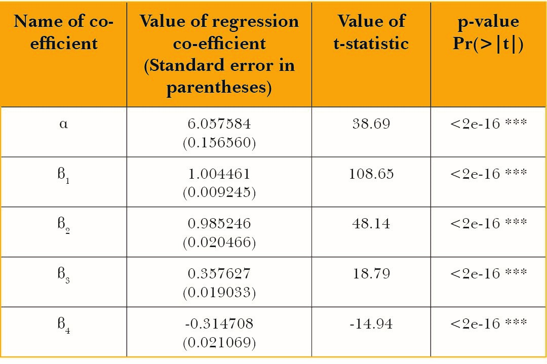
Signif. codes:  0 ‘***’ 0.001 ‘**’ 0.01 ‘*’ 0.05 ‘.’ 0.1 ‘ ’ 1
Adjusted R² of the regression: 0.9968

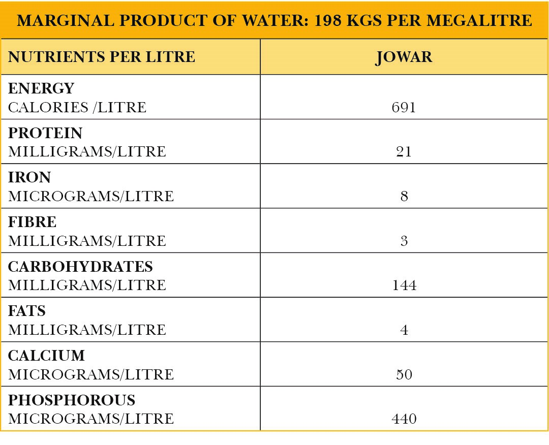
The diagnostic tests run on the residuals of the regression exhibit no autocorrelation, homoskedasticity and normality of residuals. Results are presented in the appendix. The regression co-efficient β₂ is the production elasticity of water input which equals 0.98. Multiplying this by the average product of water gives the marginal product of water which is equal to 198 kgs per megalitre of water. The marginal product in terms of nutrients contained in jowar is as follows: 

Table 7: Marginal product of water in terms of terms of output as well as nutritional content of jowar

Ragi 

Table 8: Summary output for the main regression for ragi

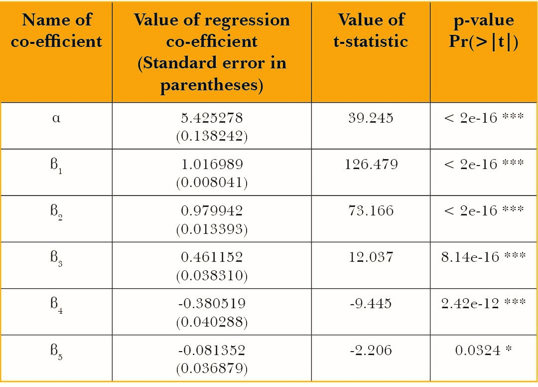
Signif. codes:  0 ‘***’ 0.001 ‘**’ 0.01 ‘*’ 0.05 ‘.’ 0.1 ‘ ’ 1
Adjusted R² of the regression: 0.9986

The diagnostic tests run on the residuals of the regression exhibit no autocorrelation, homoskedasticity and normality of residuals. Results are presented in the appendix.

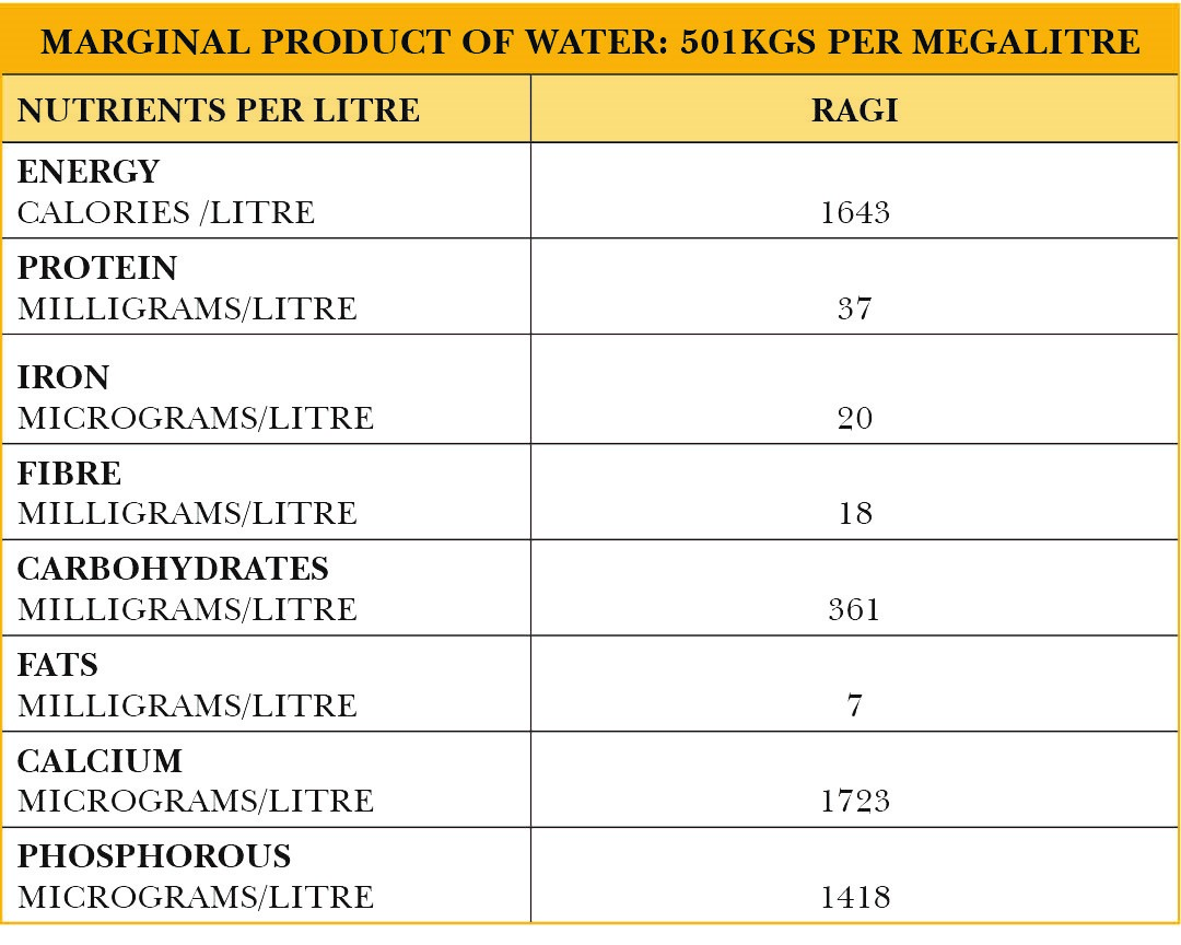
The regression co-efficient β₂is the production elasticity of water input which equals 0.98. Multiplying this by the average product of water gives the marginal product of water which is equal to 501 kgs per megalitre of water. The marginal product in terms of nutrients contained in ragi is as follows: 

Table 9: Marginal product of water in terms of terms of output as well as nutritional content of ragi

Bajra

Estimating equation (8), we get the following results:

Table 10: Summary output for the main regression for bajra

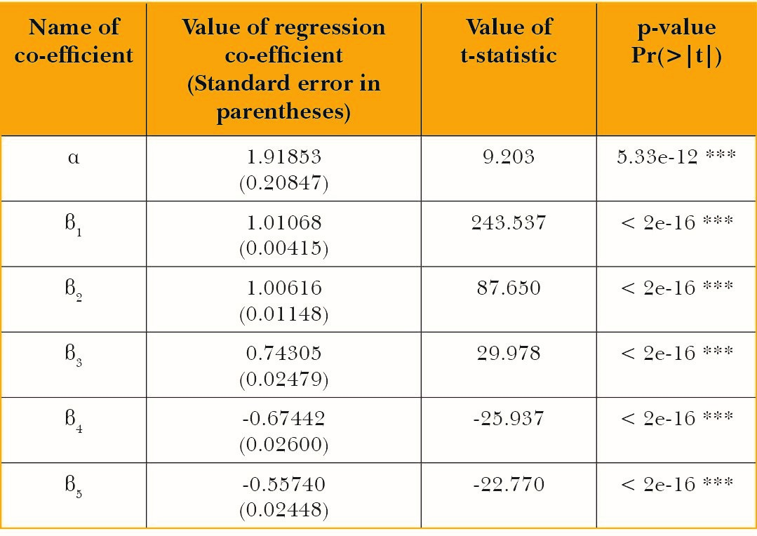
Signif. codes:  0 ‘***’ 0.001 ‘**’ 0.01 ‘*’ 0.05 ‘.’ 0.1 ‘ ’ 1
Adjusted R² of the regression: 0.9995

The diagnostic tests run on the residuals of the regression exhibit no autocorrelation, homoskedasticity and normality of residuals. Results are presented in the appendix.

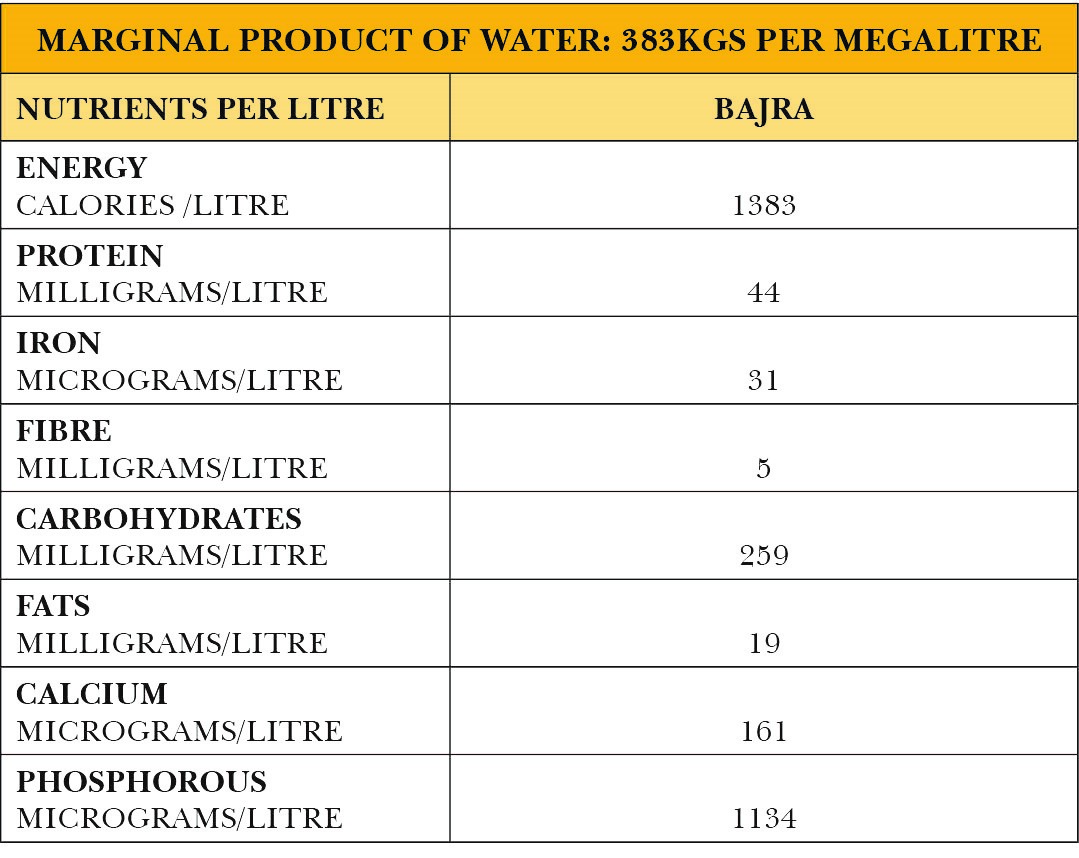
The regression co-efficient β₂is the production elasticity of water input which equals 1.01. Multiplying this by the average product of water gives the marginal product of water which is equal to 383 kgs per megalitre of water. The marginal product in terms of nutrients contained in bajra is as follows: 

Table 11: Marginal product of water in terms of terms of output as well as nutritional content of bajra

Barley

For Barley, the regression coefficient of WI_t-1is statistically insignificant. 

Table 12: Summary output for the main regression for barley

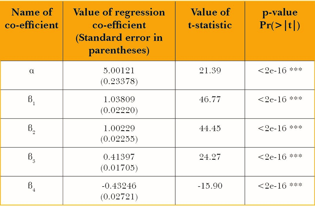
Signif. codes:  0 ‘***’ 0.001 ‘**’ 0.01 ‘*’ 0.05 ‘.’ 0.1 ‘ ’ 1
Adjusted R² of the regression: 0.9892

The diagnostic tests run on the residuals of the regression exhibit no autocorrelation, homoskedasticity and normality of residuals. Results are presented in the appendix.

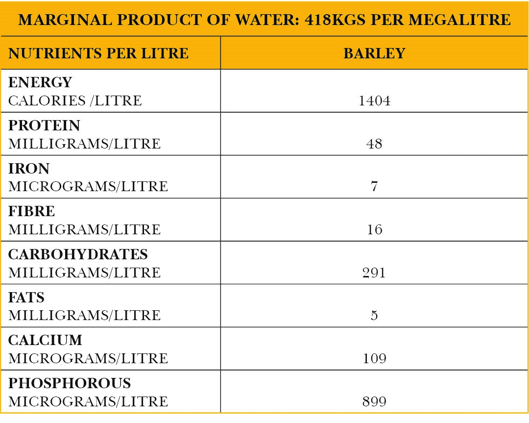
The regression co-efficient β₂is the production elasticity of water input which equals 1. Multiplying this by the average product of water gives the marginal product of water which is equal to 418 kgs per megalitre of water. The marginal product in terms of nutrients contained in barley is as follows: 

Table 13: Marginal product of water in terms of terms of output as well as nutritional content of barley

Maize

For maize, the regression coefficient of WI_t-1is statistically insignificant. 

Table 14: Summary output for the main regression for maize

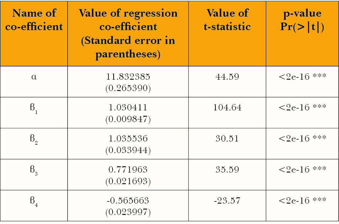
Signif. codes:  0 ‘***’ 0.001 ‘**’ 0.01 ‘*’ 0.05 ‘.’ 0.1 ‘ ’ 1
Adjusted R² of the regression: 0.996

The diagnostic tests run on the residuals of the regression exhibit no autocorrelation, homoskedasticity and normality of residuals. Results are presented in the appendix.

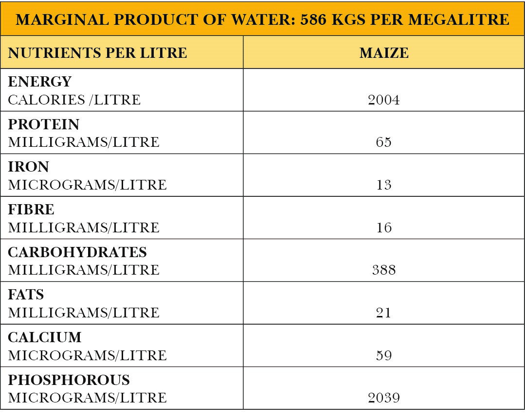
The regression co-efficient β₂is the production elasticity of water input which equals 1.03. Multiplying this by the average product of water gives the marginal product of water which is equal to 586 kgs per megalitre of water. The marginal product in terms of maize’s calorific value is as follows: 

Table 15: Marginal product of water in terms of terms of output as well as nutritional content of maize

Estimates and Discussion

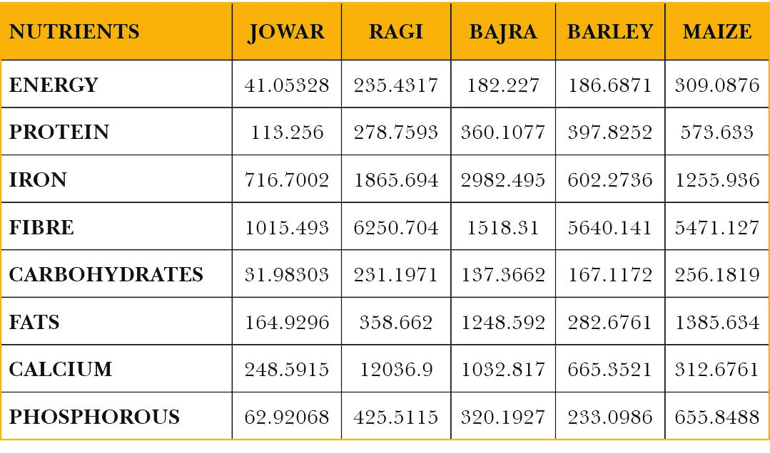
Table 16 is based on the marginal product of water in terms of various nutrients in the context of different crops. These measures reflect the productivity of water in terms of producing various nutrients when applied to the cultivation of different crops. As such, the table inform us about how efficient different crops are in producing various nutrients.

Table 16: The marginal product of water used in the production of various crops in terms of their nutrients

It is clear from the table that maize is the most efficient water user in producing calories, followed by ragi and wheat. As far as production of protein is concerned, maize is the most water-efficient followed by wheat, barley and bajra. In the context of iron, bajra followed by wheat and ragi are the better performers in terms of water efficiency in producing iron. For the case of fibre, ragi is the most water efficient, followed by barley and maize, demonstrating the same water efficiency. Maize is the most efficient water user in producing carbohydrates, with ragi being second and wheat, third. With reference to fat production, maize ranks first in water efficiency followed by bajra, and then by ragi and wheat which tie for the third position. Ragi is the best performer in the case of calcium production, with wheat being a distant second and bajra third. Maize is the most efficient water user in producing phosphorous, with wheat ranking second and ragi, third.

Ragi and maize appear several times in one of the top three ranks as efficient water users as far as the production of all the nutrients are concerned. These crops appear as the more efficient water users in nutrient production. Rice is the least efficient water user in nutrient production given that it consistently ranks last in this regard in the case of all nutrients.

Millets have been underutilised despite its potential to contribute to food security and nutritional value. Millet grains are drought-resistant crop, yield good productivity in the areas with water scarcity, along with being a ‘food medicine’.^[36] Millets are source of antioxidants and help enhance capability of probiotics with potential health benefits.^[37] Millets play a role in body immune system, a solution to tackle childhood undernutrition and iron deficiency anaemia.^[38] Evidence on nutritive value of rice vs millet shows millets to be superior not only in energy but protein, fat and fiber content as to rice.^[39]

In what follows, we calculate the nutritional gains made by transferring a megalitre of water from rice cultivation to an alternative crop. This analysis assumes land extensification when such transfer takes place. This assumption is required because, given that crop water requirement is highest in the case of rice, transferring a megalitre of water from rice cultivation to the cultivation of an alternative crop will require bringing more land under cultivation of that alternative crop when compared with rice cultivation to expend all of the transferred megalitre. Since rice is both a kharif and a rabi crop, we can consider transfers to both kharif and rabi crops. The percentage nutrient gains from such transfer to the cultivation of different alternative crops is tabulated below: 

Table 17: Percent gains in nutrient production from a transfer of a megalitre of water from rice cultivation to the cultivation of an alternative crop

As can be seen in Table 17, rice being the least efficient water user has entailed in only significant gains and no losses in nutrient production following a transfer of a megalitre of water from rice to alternative crop production.

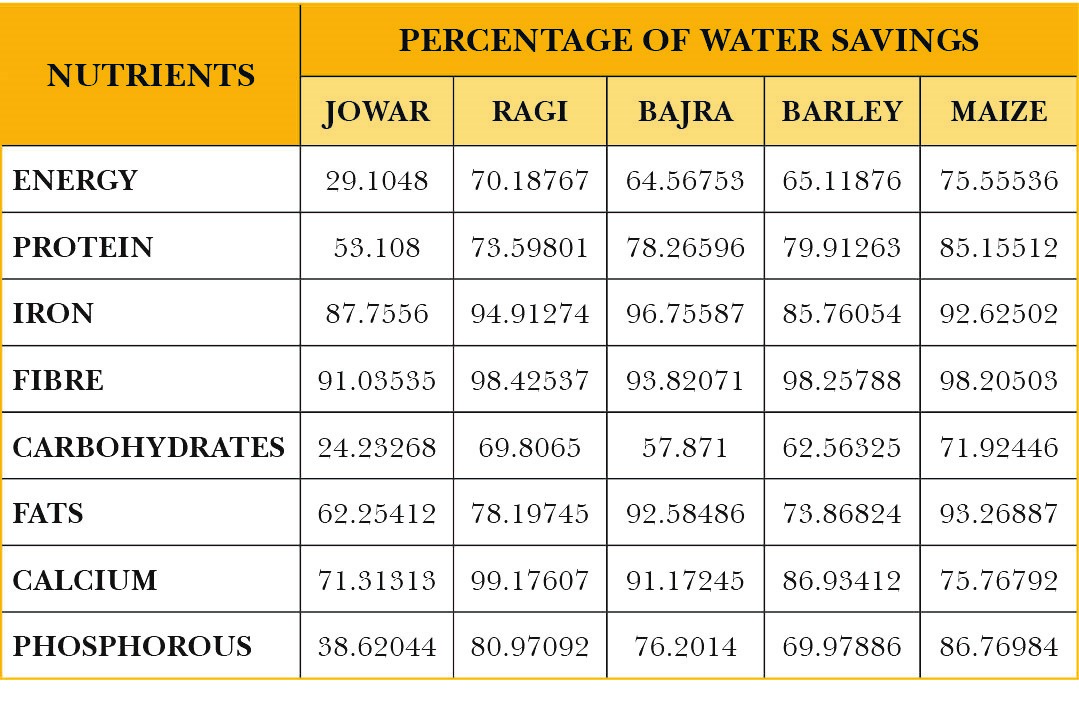
Consider a situation in which the same amount of nutrients contained in rice yielding from one megalitre of water is produced but this is done by shifting the cultivation to an alternative crop. We compute the water savings resulting from this situation. Production of the same amount of nutrients by transferring cultivation from rice to another crop may require land under cultivation to be either held constant or reduced.

Table 18: Percentage of water reduced in producing the same amount of nutrients yielding from rice cultivation by shifting to alternative crop cultivation

In what follows, the analysis measures the percentage gains in nutrient production resulting from shifting a certain proportion of the acreage under rice cultivation to cultivation under alternative crops. It must be noted that the resulting percentage gains in nutrient production due to a shift to an alternative crop is the same irrespective of the proportion acreage transferred. Here a proportion of the rabi acreage under rice cultivation is assumed to be shifted to other rabi crops such as jowar, maize and barley. Also, a proportion of the annual acreage of the rice cultivation is assumed to be shifted under ragi cultivation.

Table 19: Percentage gains in nutrient production due to a shift of acreage from rice cultivation to an alternative crop

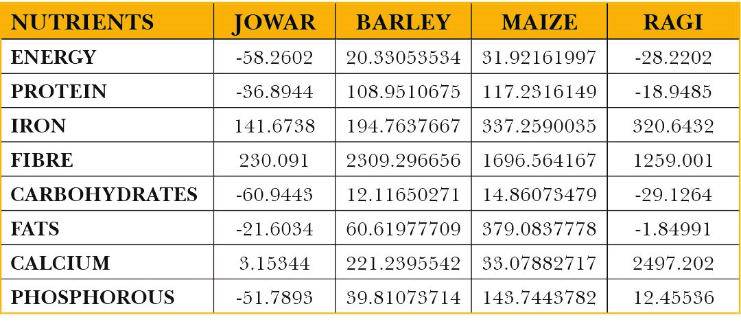
When a proportion of acreage under rice is shifted to jowar cultivation, there is a significant loss in nutrient production in all but three nutrients namely iron, fibre and calcium. A similar shift to maize cultivation results in gains in the production of all nutrients. In case of shift to barley cultivation, there is an increase in the production of all nutrients. A shift to ragi production also results in increase in iron, fibre, calcium and phosphorous but a decline in calories, proteins, carbohydrates and fats. While shifts to alternative crop cultivation does yield significant increases in nutrient production, there are losses that are registered. Whether these losses can be afforded depends upon what implications such losses have for nutritional security.

In what follows, the table presents the water savings resulting from the above exercise of shifting acreage under rice cultivation to other alternative crops. The percentage savings remains the same irrespective of the acreage under rice shifted to other crops.

Table 20: Percentage of water savings from shifting acreage under rice cultivation to other crops 

Policy Implications

Being under severe water stress, India is among nations characterised by extremely fragile water resources in the world. With agriculture being the dominant water user, opportunities within the sector to improve water -use efficiency need to be exploited. One such opportunity is presented by the water intensive crop cultivation patterns in India. This paper explores the implications of replacing this water intensive cropping pattern with less water consuming crops on nutritional gains and water savings. The discussion in this paper is based on a notion of water productivity defined as the marginal product of water. This marginal product quantifies the additional output generated and the nutrients produced by applying an additional unit of water input (here, megalitre) to the cultivation of a given crop.

The investigation in this paper finds that rice is the least efficient water user in nutrient production, while ragi and maize emerge consistently as water efficient crops in terms of nutrient production. Furthermore, the analysis reveals that replacing rice cultivation by transferring a unit of water input, here megalitre, which entails shifting of acreage from rice cultivation to alternative actually results in gains in nutrient production and water savings too. Furthermore, the analysis reveals that shifting acreage from rice cultivation to other alternative crops results in nutrient gains only in case of maize and barley, but both nutrient gains and losses in case of shift in cultivation to jowar and ragi. However, such shift from rice cultivation to other crops results in water savings and no water losses in all cases.

As a fillip to the Sahi Fasal water campaign, policymakers need to take note of the gains in nutrient production and water savings resulting from the shift to an alternative regime of cropping patterns. This paper makes the following recommendations to encourage farmers to replace rice cultivation with better alternatives:

1. Rice and wheat enjoy a guaranteed minimum support price and assured markets through procurement as well as significant consumer subsidies through the Public Distribution System. This makes the production of these crops remunerative, generating high economic yields. This incentivises the production of these water consuming crops against that of less water intensive crops which are also more efficient in nutrient production. There is a need to create such economic incentives in favour of less water-intensive crops so that farmers are encouraged to produce them.
2. The above-mentioned water guzzlers are dominantly produced in water-scarce regions in the presence of perverse incentives such as concessional or free supply of electricity and lack of appropriate water pricing. A push in the direction of water-efficient crops can be expected if such incentives are done away with to be replaced by appropriate pricing of irrigation water and electricity. Prices must at the least cover operation and maintenance costs.
3. For improved water use efficiency, the cultivation of alternatives to rice and wheat needs to be aligned with their suitability of cultivation in terms of agro-climatic-hydro conditions prevailing across diverse geographical zones in the country. Research that identifies such mapping needs to be encouraged.
4. To further enhance the water efficiency of nutrient production resulting from alternative crop cultivation, there is a need to identify the most optimal and efficient irrigation strategy for such alternative cropping regimes.
5. Smart varieties of alternative crops that perform well under water-stress and drought conditions may be developed to further augment the gains in water efficiency.
6. Best farm management practices that can increase the yield of less water consuming crops can ensure the expected gains from the cultivation of these crops.
7. While farmers are made aware of the benefits of cultivating less water-consuming, nutrition-rich alternatives, there is a need for creating awareness among consumers to also switch to these alternatives.

At the same time, it needs to be acknowledged that there are issues with the marketing of the millets, as the market size is presently small, and the product has a short shelf life depending on humidity and temperature. Of course, the government needs to intervene through three ways: to promote the crop through price signals (increase MSPs, and promote the crops through lower pricing at the public distribution shops); create awareness of the nutritional values; and set up better storage facilities for the crop for increasing its longevity. However, the agricultural marketing question is beyond the scope of this paper, and will require a separate analysis altogether.

On the other hand, there are again concerns with consumer choice. A large majority of the consumers in India and other countries prefer consuming paddy because of ease of cooking and also because of their habits. There may also be questions on how nutritious the cooking mechanism is as certain food items might require more oil than others. More awareness creation drives, and at times, price incentives need to be created to encourage a shift in consumer choices.  These questions are also outside the scope of this paper.

Conclusion

Implementing the recommendations outlined in this paper can help mitigate the intensity of the water crisis confronting India. It is imperative that the calculus of productivity now expands to incorporate the concerns of water productivity along with that of land and the economy. This is expected to make the global food production system more sustainable and resource-efficient.

This paper underlines the criticality of crop choice for future water security on one hand, and nutritional security on the other. In other words, there are backward and forward linkages associated with the kind of crops that the nation grows. From a water security perspective, it is the backward linkages with the choice of food crops. This is related to the broader sustainability aspect of ecosystem, apart from human and economic needs of water. Agricultural expansion during the last century has caused widespread changes in land cover, watercourses, and aquifers, as well as the flow regime as a whole, inhibiting the capacity to provide for the provisioning services of the ecosystem.^[40] While technological interventions made more water available for irrigation thereby promoting production of water-intensive crops, such a practise has threatened the ecological foundation of the food system.^[41]

Unfortunately, the management policy of many agro-ecosystems has essentially been based on the premise that they are delinked from the broader landscape. There has been scant recognition of the ecological components and the processes that support the sustainability of such agro-ecosystems. The carrying capacity of the ecosystem has thus been defied by traditional agricultural and water management regimes. Some ecosystems were made to cross the ecological thresholds, leading to a regime change in the ecosystem and their concomitant services. The resultant reduction in the ecosystem’s resilience also restricts the sustainability of its food provisioning service. Beyond a point, even the water supply augmentation plans (through dam constructions), and land-use change (entailing bringing more land under agriculture by cutting down forests or filling wetlands), do not work and can have a negative impact on food security.

India’s penchant for water consuming crops is discernible from the fact that the Green Revolution in the 1960s was mostly successful in the context of paddy and wheat. As such, India’s food security has largely been delineated through production and distribution of rice and wheat. This leads to choosing economic instruments like the MSP that incentivise the cultivation of water-intensive crops over indigenous, water-efficient crops of the region. This increases the competing demands for water over a long period, further aggravating the water conflicts in India.

The acknowledgement of the need for a holistic approach to manage water and govern river basins is reflected in recent policy documents and the actions of the developed world.^[42] The spree of dam decommissioning is testimony to the changing paradigm that gives higher priority to projects that meet basic and unmet human and ecosystem needs for water.^[43]

This is increasingly being recognised by the emerging paradigm of Integrated Water Resources Management (IWRM). With these types of changes occurring all across the world, the new paradigm that looks at water from a broader landscape or basin ecosystem perspective, delinks the relation between water and food security. In other words, ever increasing supply of water is no longer a necessary condition for food security, but better demand management of water can help reconcile food and water security, while keeping water instream for ecosystem concerns.

At the next stage emerges the forward linkage with nutritional security that is largely contingent on the choice of food. This paper attempted to rationalise water use from the perspective of producing better food. While it is clear that from the perspective of nutrition, water use is not optimised in India, the need for promoting alternative crops has been highlighted by the numbers that this analysis has estimated in terms of productivity. There is no doubt that in India, a reductionist approach has been followed to promote nutritional security without concerning itself with the fundamental basis of production processes. This paper does not deal with the distribution aspect of nutrition. However, when the supply-side is being taken care of through better procurement prices of more nutritional crops, that can often release the demand-side pressures that may create access problems for consumers.

From the UN Sustainable Development Goals perspectives, this has four implications. First, from the perspective of SDG 2 (Zero Hunger), this paper not only has implications for food security, but also for improved nutrition, and promotion of sustainable agriculture by rationalising the use of natural capital While it is often stated that land, water, and plant genetic resources are key inputs into food production, it is often a flow regime of a basin ecosystem that supports the land, soil and genetic diversity. It has also been argued that producing alternative drought-resistant crops can help realise more farm incomes thereby helping farmer’s well-being and rural development.^[44] Second, from the perspective of SDG 1 (No Poverty), this research talks of demand-management of water for keeping water instream that helps in maintaining the integrity of the basin ecosystem. This will help in provision of the ecosystem services that are also called “GDP of the poor”^[45] because of their contributions to the lives and livelihoods of the poor. Third, it plays a role in mitigation and adaptation to climate change for achieving SDG 13 (Climate Action) and also has implications for SDG 15 (life on land) as natural capital and terrestrial ecosystem can be supported with maintaining flow regimes. Fourth, such demand-side interventions are crucial for incentivising farmers to shift their cropping patterns. Such shift will be in the nature of promoting SDG 12 (responsible production and consumption). Cultural and other factors affecting dietary choices need to be fully understood in formulating an effective behaviour change campaign. This research can pave the way for an integrated approach to water-food-energy (nutrition, in this case) nexus, thereby helping the cause of human well-being and ecosystems sustainability.

APPENDICES

 A.1. Blaney Criddle Method:

Monthly crop water need: ETCROP (mm/month) =

ETO(mm/day)x Kc x number of days in a month dedicated to the growing season

Where:

ET_CROP: Crop Evapotranspiration or crop water need

ET_O: Reference Evapotranspiration

Kc: Crop factor for a particular growth stage

Total crop water need (mm) =

ΣMonthly crop water need (mm/month) Where the summation is over all the months belonging to the various growth stages of the crop

India-adjusted total crop water need for each year from 1967 to 2019=

(Total crop water need for a year/ Maximum across total annual crop water need from 1967 to 2019) xIndia-specific crop water need

A.2. Identification of components of non-stationarity and memory

1. Wheat

The components of non-stationarity have to be identified for the logarithmic transformation of the variables of wheat production, yield of wheat and water unput for wheat production.

• The case of wheat production

Table 21: Results of ADF test with drift and linear trend for the case of wheat production

Statistic	Value of the statistic	Statistical significance
Tau (τ) statistic	-3.0793	Statistically insignificant
Statistic associated with drift (constant term)	9.0915	Statistically significant at 1 percent level
Statistic associated with linear trend term	6.6288	Statistically significant at 5 percent level

The variable of wheat production contains a unit root and there is evidence that it also contains a linear trend term. Let us confirm using a regression-based test.

Log_WP_t = α+β₁Log_WP_t-1+β₂t+ e_t

Where Log_WP_t: Logarithmic transformation of wheat production in the t^th year

Log_WP_t-1: Logarithmic transformation of wheat production in the t-1^th year

t: Linear trend term

e_t: error term

Running the above regression yields the following result:

Table 22: Summary output of the regression-based test for confirming the existence of unit root and linear trend in the stochastic process of wheat production

Name of co-efficient	Value of co-efficient (Standard error in parentheses)	Value of t-statistic	p-value Pr(>|t|)
Α	7.678935 (1.567199)	4.900	1.09e-05 ***
β1	0.680109 (0.066038)	10.299	7.51e-14 ***
β2	0.009117 (0.002333)	3.908	0.000285 ***

Signif. codes:  0 ‘***’ 0.001 ‘**’ 0.01 ‘*’ 0.05 ‘.’ 0.1 ‘ ’ 1

Adjusted R² of the regression: 0.9796

This suggests that the variable of wheat production contains both a unit root and a linear trend.

When various combinations of non-stationarity components are checked, the results suggest that along with the unit root and the linear trend, the quadratic trend is also statistically significant When the quadratic trend is included to run the following regression,

Log_WP_t = α+β₁Log_WP_t-1 +β₂t+β₃t²+ e_t,

Where t²: quadratic trend term

we obtain the following results:

Table 23: Summary output of the finalised regression-based test capturing all components of non-stationarity and memory for the stochastic process of wheat  production

Name of co-efficient	Value of co-efficient (Standard error in parentheses)	Value of t-statistic	p-value Pr(>|t|)
α	1.470e+01 (2.428e+00)	6.055	2.07e-07 ***
β1	3.786e-01 (1.036e-01)	3.654	0.000638 ***
β2	3.393e-02 (7.294e-03)	4.652	2.61e-05 ***
β3	-2.755e-04 (7.757e-05)	-3.552	0.000870 ***

Signif. codes:  0 ‘***’ 0.001 ‘**’ 0.01 ‘*’ 0.05 ‘.’ 0.1 ‘ ’ 1

Adjusted R² of the regression:0.9835

For the residuals of this regression, the Durbin-Watson test statistic for the alternative hypothesis of autocorrelation not equal to zero equals 1.9309 and the associated p-value equals 0.5253

This suggests that the wheat production is not only composed of an autoregressive unit root and a linear trend, but also a quadratic trend. While extracting the unit root and the linear trend may render the variable stationary, it would have contained traces of past information. By identifying the existence of the quadratic trend, we can detrend the series to get rid of this past information as well.

• The case of wheat yield

Table 24: Results of ADF test with drift and linear trend for the case of wheat yield

Statistic	Value of the statistic	Statistical significance
Tau (τ) statistic	-2.3991	Statistically insignificant
Statistic associated with drift (constant term)	6.1321	Statistically significant at 5 percent level
Statistic associated with linear trend term	3.4683	Statistically insignificant

The results of ADF test indicate the presence of a unit root in the stochastic process of wheat yield. While undertaking the confirmatory investigation utilising the regression test, it is checked whether there are other sources of non-stationarity or past information in the stochastic process. Even if a source of non-stationarity is individually statistically insignificant but accounts for a fraction of adjusted R² of the regression, we retain that source or component. In the case of wheat yield, it is revealed that a unit root, linear trend and a quadratic trend are statistically significant and explain non-stationarity, memory and traces of past information. While differencing or de-memorising the stochastic process may have rendered it stationary, detrending enables extracting out all of the non-stationarity and the past information contained in the process.

In the case of wheat yield, the following regression has been finalised as capturing the components of non-stationarity in it:

Log_WY_t = α+β₁Log_WY_t-1 +β₂t+β₃t²+ e_t,

Where:

Log_WY_t: Logarithmic transformation of wheat yield in the t^th year

Log_WY_t-1: Logarithmic transformation of wheat yield in the t-1^th year

Table 25: Summary output of the finalised regression-based test capturing all components of non-stationarity and memory for the stochastic process of wheat yield

Name of co-efficient	Value of co-efficient (Standard error in parentheses)	Value of t-statistic	p-value Pr(>|t|)
α	4.399e+00 (8.963e-01)	4.908	1.1e-05 ***
β1	3.711e-01 (1.303e-01)	2.848	0.006452 **
β2	2.284e-02 (5.860e-03)	3.898	0.000301 ***
β3	-1.856e-04 (6.198e-05)	-2.995	0.004332 **

Signif. codes:  0 ‘***’ 0.001 ‘**’ 0.01 ‘*’ 0.05 ‘.’ 0.1 ‘ ’ 1

Adjusted R² of the regression:0.9835

For the residuals of the above regression, the Durbin-Watson test statistic for the alternative hypothesis of autocorrelation not equal to zero equals 1.7891 and the associated p-value equals 0.2574.

• The case of water input for wheat production

Table 26: Results of ADF test with drift and linear trend for the case of water input for wheat production

Statistic	Value of the statistic	Statistical significance
Tau (τ) statistic	-3.9264	Statistically significant at 5 percent level
Statistic associated with drift (constant term)	8.3158	Statistically significant at 1 percent level
Statistic associated with linear trend term	9.5135	Statistically significant at 1 percent level

The ADF results suggest that the stochastic process underlying water input of wheat production is stationary and has a linear trend. Confirming this result involves running the following regression:

Log_WI_t = α+β₁t+ e_t

Where:

Log_WI_t: Logarithmic transformation of water input for wheat production in the t^th year

Table 27: Summary output of the regression-based test for confirming the existence of trend term in the stochastic process of the water input used in wheat production

Name of co-efficient	Value of co-efficient (Standard error in parentheses)	Value of t-statistic	p-value Pr(>|t|)
α	1.851e+01 (1.649e-02)	1122.30	<2e-16 ***
β1	1.188e-02 (5.414e-04)	21.94	<2e-16 ***

Signif. codes:  0 ‘***’ 0.001 ‘**’ 0.01 ‘*’ 0.05 ‘.’ 0.1 ‘ ’ 1

Adjusted R² of the regression:0.9041

Although the adjusted R² of the regression is as high as 0.9041, the Durbin-Watson test statistic for the alternative hypothesis of autocorrelation not equal to zero equals 0.45463and the associated p-value equals 1.283e-12. This high autocorrelation in the residuals is evident even in the correlogram representing these residuals.

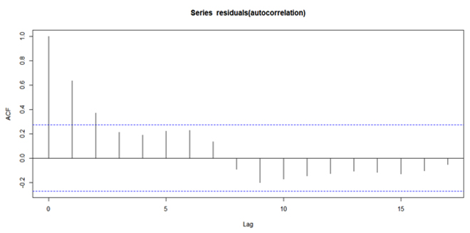
Figure 1: Correlogram (Autocorrelation Function) of the residuals from the regression which includes only trend as a component of non-stationarity

It is clear that the linear trend alone does not exhaustively capture the memory and the non-stationarity exhibited by the stochastic process underlying the water input used for wheat production. Exploratory regression-based tests indicate that adding an autoregressive term and a quadratic trend significantly explains the memory and the non-stationarity in the stochastic process under consideration although the autoregressive term is statistically significant while the quadratic trend is not. Nevertheless, since the inclusion of the quadratic trend term adds to the adjusted R², it is retained in the regression equation which will be used as the basis for rendering the process stationary.

The above-mentioned regression takes the form:

Log_WI_t = α+β₁Log_WI_t-1 +β₂t+β₃t²+ e_t,

Where:

Log_WI_t: Logarithmic transformation of water input for wheat production in the t^th year

Log_WI_t-1: Logarithmic transformation of water input for wheat production in the t-1^th year

Running the above regression yields the following results:

Table 28: Summary output of the finalised regression-based test capturing all components of non-stationarity and memory for the stochastic process of water input used in wheat production

Name of co-efficient	Value of co-efficient (Standard error in parentheses)	Value of t-statistic	p-value Pr(>|t|)
α	7.231e+00 (1.474e+00)	4.906	1.11e-05 ***
β1	6.098e-01 (8.025e-02)	7.598	8.97e-10 ***
β2	5.844e-03 (2.288e-03)	2.554	0.0139 *
β3	-3.326e-05 (2.841e-05)	-1.171	0.2475

Signif. codes:  0 ‘***’ 0.001 ‘**’ 0.01 ‘*’ 0.05 ‘.’ 0.1 ‘ ’ 1

Adjusted R² of the regression:0.969

For the residuals of the above-mentioned regression, the Durbin-Watson test statistic for the alternative hypothesis of autocorrelation not equal to zero equals 1.9077 and the associated p-value equals0.4496. The associated correlogram representing the residual of the mentioned regression is as follows:

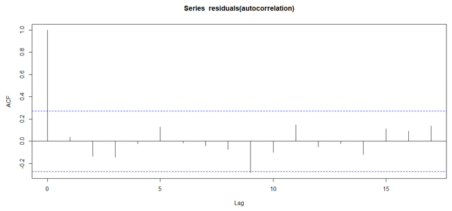
Figure 2: Correlogram (Autocorrelation Function) of the residuals from the regression which includes unit root, trend and quadratic trend as components of non-stationarity

A.3. Results of stationarity tests after the variables to be included in the main regression for computing the marginal product of water have been rendered stationary

Table 29: Results of stationarity tests after the variables have been rendered stationary (ADF with drift for current variables and ADF with no drift and no trend for lagged variables)

Name of the variable	Value of the tau (τ) statistic
Current wheat production	-4.5275
Current wheat yield	-4.4223
Current water input for wheat production	-5.379
Lagged wheat production	-3.8074
Lagged wheat yield	-3.8421
Lagged water input for wheat production	-3.4071
Current rice production	-4.0872
Current rice yield	-3.8083
Current water input for rice production	-4.2227
Lagged rice production	-4.399
Lagged rice yield	-3.9689
Lagged water input for rice production	-3.9569
Current jowar production	-5.261
Current jowar yield	-5.2494
Current water input for jowar production	-4.4614
Lagged jowar production	-4.3772
Lagged jowar yield	-4.4452
Lagged water input for jowar production	-2.9821
Current ragi production	-5.8072
Current ragi yield	-5.6981
Current water input for ragi production	-4.404
Lagged ragi production	-5.7519
Lagged ragi yield	-6.0906
Lagged water input for ragi production	-3.3507
Current bajra production	-5.4036
Current bajra yield	-5.6669
Current water input for bajra production	-4.4323
Lagged bajra production	-5.9714
Lagged bajra yield	-5.869
Lagged water input for bajra production	-4.6161
Current barley production	-4.6619
Current barley yield	-4.1314
Current water input for barley production	-4.4218
Lagged barley production	-3.8462
Lagged barley yield	-4.1093
Lagged water input for barley production	-2.4765
Current maize production	-5.6671
Current maize yield	-5.7245
Current water input for maize production	-4.5383
Lagged maize production	-6.4258
Lagged maize yield	-5.804
Lagged water input for maize production	-3.0958

Except for the lagged water input for barley production for which the tau (τ)statistic is statistically significant at 5 percent level, this statistic, for all other variables, is statistically significant at 1 percent level. This implies stationarity of all the current and lagged variables considered in the above-mentioned table.

A.4. Diagnostics run on the residuals of the main regression model of the crops under study

Table 30: Diagnostics run on the residuals of wheat’s main regression model

Type of test	Value of statistic	p-value	Conclusion
Box-Pierce autocorrelation test	0.90061	0.3426	Residuals show no autocorrelation
Breusch-Pagan homoskedasticity test	2.284	0.6837	Residuals are homoscedastic
Shapiro-Wilk normality test	0.9789	0.4803	Residuals are normal

Table 31: Diagnostics run on the residuals of rice’s main regression model

Type of test	Value of statistic	p-value	Conclusion
Box-Pierce autocorrelation test	1.2817	0.2576	Residuals show no autocorrelation
Breusch-Pagan homoskedasticity test	2.5517	0.6354	Residuals are homoscedastic
Shapiro-Wilk normality test	0.96886	0.1889	Residuals are normal

Table 32: Diagnostics run on the residuals of jowar’s main regression model

Type of test	Value of statistic	p-value	Conclusion
Box-Pierce autocorrelation test	0.21592	0.6422	Residuals show no autocorrelation
Breusch-Pagan homoskedasticity test	4.1371	0.3878	Residuals are homoscedastic
Shapiro-Wilk normality test	0.9742	0.3158	Residuals are normal

Table 33: Diagnostics run on the residuals of ragi’s main regression model

Type of test	Value of statistic	p-value	Conclusion
Box-Pierce autocorrelation test	3.0967	0.07845i	Residuals show no autocorrelation
Durbin-Watson Test (Alternative hypothesis: True autocorrelation is not equal to zero)	2.487	0.1245	Residuals show no autocorrelation
Breusch-Pagan homoskedasticity test	2.3922	0.7926	Residuals are homoscedastic
Shapiro-Wilk normality test	0.97186	0.2529	Residuals are normal

ⁱSince the evidence of no autocorrelation is weak in case of the Box-Pierce test, the Durbin-Watson test is carried out which lends credence to the conclusion of no autocorrelation

Table 34: Diagnostics run on the residuals of bajra’s main regression model

Type of test	Value of statistic	p-value	Conclusion
Box-Pierce autocorrelation test	1.7418	0.1869	Residuals show no autocorrelation
Breusch-Pagan homoskedasticity test	4.8399	0.4357	Residuals are homoscedastic
Shapiro-Wilk normality test	0.95867	0.06853ii	Residuals are normal
Jarque-Bera test of normality	2.7809	0.249	Residuals are normal

ⁱⁱ Since the evidence of normality of residuals is weak in case of the Shapiro-Wilk normality test, the Jarque-Bera test of normality is carried out which lends credence to the conclusion of normality of residuals

Table 35: Diagnostics run on the residuals of barley’s main regression model

Type of test	Value of statistic	p-value	Conclusion
Box-Pierce autocorrelation test	0.79021	0.374	Residuals show no autocorrelation
Breusch-Pagan homoskedasticity test	1.2134	0.8759	Residuals are homoscedastic
Shapiro-Wilk normality test	0.98284	0.6528	Residuals are normal

Table 36: Diagnostics run on the residuals of maize’s main regression model

Type of test	Value of statistic	p-value	Conclusion
Box-Pierce autocorrelation test	2.3016	0.1292	Residuals show no autocorrelation
Breusch-Pagan homoskedasticity test	8.9379	0.06267iii	Residuals are homoscedastic
Goldfeld-Quandt test	1.6688	0.2488	Residuals are homoscedastic
Shapiro-Wilk normality test	0.98446	0.7271	Residuals are normal

ⁱⁱⁱ Since the evidence of homoskedasticity is weak in the case of the Breusch-Pagan homoskedasticity test, the Goldfeld-Quandt test is carried out which lends credence to the conclusion of homoskedasticity of residuals.

Endnotes

• Water
• Agriculture
• India
• agriculture
• Climate change
• INDIA
• occasional papers
• Sustainable development
• water

The views expressed above belong to the author(s). ORF research and analyses now available on Telegram! Click here to access our curated content — blogs, longforms and interviews.